Segmentation Strategies and Window Design
Preprocessing is not only about cleaning EEG. It also defines the unit that the model will see. In affective computing, segmentation choices determine how much temporal context is preserved, how labels are assigned, how many training samples are created, and whether evaluation is vulnerable to leakage. For that reason, window design is both a preprocessing issue and a modeling assumption.
This section discusses how segmentation choices interact with affective EEG tasks, especially when moving between batch prediction and online continuous prediction.
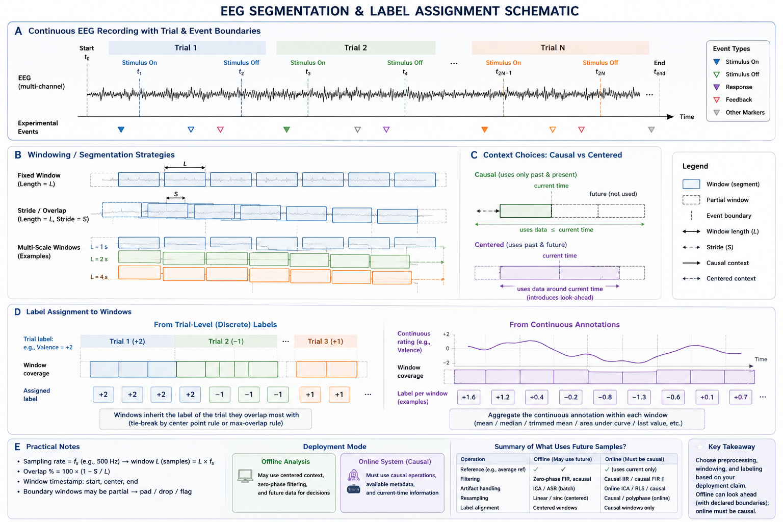
Figure 6.3: EEG segmentation and label assignment. Window length, stride, overlap, alignment, and label inheritance determine the temporal context and statistical dependence of the examples supplied to a model.
Why Segmentation Matters
EEG recordings are usually longer and more irregular than the fixed-size tensors expected by many learning algorithms. Segmentation converts a continuous signal into training examples, but that conversion is not neutral. A five-second window with 50% overlap expresses a very different assumption from a one-second causal window with no overlap.
Windowing affects at least four things simultaneously:
| Design choice | Main consequence |
|---|---|
| Window length | Controls temporal context and stationarity assumptions |
| Window overlap | Controls sample density and leakage risk |
| Alignment strategy | Controls whether the segment reflects onset, steady state, or recovery |
| Label assignment | Controls what target the model is actually trained to predict |
Because of this, segmentation should be justified relative to the target task rather than treated as a fixed preprocessing default.
Fixed-Length Windows
Fixed-length windowing is the most common strategy. The signal is divided into segments of equal duration, often with some overlap, and each segment is treated as an input sample. This works well for conventional deep learning pipelines and makes batching straightforward.
The main tradeoff is between context and specificity. Longer windows provide richer temporal information and can stabilize spectral estimates, but they may blur brief affective changes and increase response latency. Shorter windows are more responsive, yet they may be noisier and less informative.
In practice, window length should be chosen with the intended task in mind. Offline batch classification may tolerate or even benefit from longer windows, while online tracking usually requires shorter, causal segments.
Overlapping Windows
Overlap is commonly used to increase the number of training examples and to smooth predictions over time. However, overlap introduces one of the most important sources of evaluation leakage in EEG studies. If overlapping windows derived from the same continuous interval are split across training and testing, the test set may contain samples that are nearly duplicates of training samples.
The consequences are especially severe in within-subject and within-trial evaluation. Overlap itself is not wrong, but it must be handled consistently with the train-test protocol.
| Overlap policy | Benefit | Risk |
|---|---|---|
| No overlap | Clean independence between windows | Fewer samples, lower temporal resolution |
| Moderate overlap | Denser sampling and smoother trajectories | Leakage if split after segmentation |
| Heavy overlap | Large sample count and fine-grained updates | Strong sample redundancy and inflated scores |
Event-Aligned and State-Aligned Segmentation
Not all segments need to be uniform sliding windows. In some datasets, it is meaningful to align windows to stimulus onset, response onset, or annotated change points. Event-aligned segmentation is useful when the task concerns transient affective responses, such as reactions to clips, feedback, or specific interactive moments.
State-aligned segmentation, in contrast, aims to capture relatively stable intervals of affect and may be more appropriate for sustained emotion tracking. The distinction matters because onset-focused windows emphasize dynamics, while state-centered windows emphasize persistence.
Adaptive and Multi-Scale Segmentation
Fixed windows are convenient, but affective EEG does not always change at a fixed rate. Adaptive segmentation uses signal changes, event boundaries, or changes in continuous annotations to define variable-duration intervals. For example, a method may place a boundary at an annotated affective transition, a stimulus change, or a detected change in spectral or spatial EEG properties.
Adaptive boundaries can avoid mixing a transient response with a later steady state, but they introduce another modeling decision: the boundary detector must be specified and evaluated without using held-out labels improperly. If a detector is learned from data, fit it on the training partition and apply it unchanged to validation and test data. For online use, the detector must use only past and present samples.
Multi-scale segmentation provides several views of the same recording, such as short windows for rapid changes and longer windows for stable spectral estimates. This can be implemented by training separate models, concatenating representations from several scales, or using a hierarchical temporal model. The approach can improve coverage of different affective time scales, but related windows must remain in the same evaluation group to prevent leakage.
| Strategy | Best suited to | Main tradeoff |
|---|---|---|
| Fixed-length windows | Standardized offline benchmarks | May not match changes in affective state |
| Adaptive intervals | Event-driven or nonstationary recordings | Boundary detection can be unstable or label-dependent |
| Multi-scale windows | Processes with fast and slow dynamics | More samples and stronger redundancy between scales |
Label Assignment Under Segmentation
Segmentation is tightly coupled to labeling. A trial-level label assigned to every short window assumes that the emotional state is constant throughout the trial. That assumption may be acceptable in some paradigms, but it is clearly questionable in others.
Common label assignment strategies include:
- inheriting the trial label for every window,
- assigning labels from temporally local annotations,
- averaging continuous labels within the window,
- or using future labels when the task is forecasting rather than state estimation.
The label rule should match the task claim. If the model is evaluated as a continuous tracker, then label assignment should respect the temporal evolution of the target rather than flattening it into a constant trial-level category.
Segmentation for Batch Versus Online Tasks
Segmentation should differ across task branches.
For batch prediction, segments may be designed to maximize discriminability and can sometimes include broader context, provided the benchmark is defined offline. For online prediction, segmentation must reflect causality: each window should only use currently available or past information, and the window size partly determines the latency of the system.
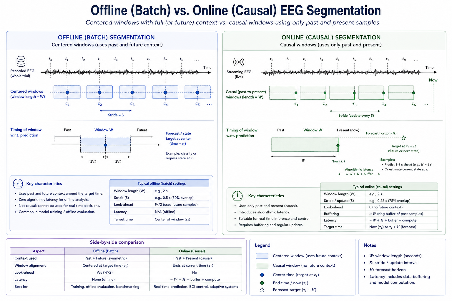
Figure 6.4: Batch versus online segmentation. A segmentation strategy valid for offline benchmarking may not support an online claim unless its context, latency, and label availability are causal.
This distinction is easy to overlook, but it is central. A segmentation strategy that is valid for offline benchmarking may not support an honest online claim.
Practical Recommendations
Several guidelines are generally useful.
- Choose window length based on the time scale of the affective process and the response latency tolerated by the application.
- If overlap is used, split data by trials, sessions, subjects, or time blocks before allowing windows from the same source interval to populate different partitions.
- State clearly whether segmentation is causal, centered, or uses future context.
- Document how labels are assigned to each segment and whether annotation delay is compensated.
- Report sensitivity analyses when possible, because performance may depend strongly on window size and stride.
Segmentation is often treated as a technical detail, but in affective EEG it is better understood as a compact statement of the temporal assumptions built into the learning problem.
References
- Bashivan, P., Rish, I., Yeasin, M., and Codella, N. (2016). Learning representations from EEG with deep recurrent-convolutional neural networks. International Conference on Learning Representations.
- Craik, A., He, Y., and Contreras-Vidal, J. L. (2019). Deep learning for electroencephalogram (EEG) classification tasks: A review. Journal of Neural Engineering, 16(3), 031001.
- Schirrmeister, R. T., Springenberg, J. T., Fiederer, L. D. J., Glasstetter, M., Eggensperger, K., Tangermann, M., Hutter, F., Burgard, W., and Ball, T. (2017). Deep learning with convolutional neural networks for EEG decoding and visualization. Human Brain Mapping, 38(11), 5391-5420.
- Shu, L., Xie, J., Yang, M., Li, Z., Li, Z., Liao, D., Xu, X., and Yang, X. (2018). A review of emotion recognition using physiological signals. Sensors, 18(7), 2074.