Recurrent Neural Networks (RNNs) and Long Short-Term Memory (LSTMs)
Overview
Recurrent Neural Networks process sequences by maintaining hidden state across time steps. Unlike CNNs that apply the same operation across the signal, RNNs process EEG data sequentially, with each time step influencing subsequent processing. Long Short-Term Memory (LSTM) networks address the vanishing gradient problem of vanilla RNNs, making them ideal for capturing long-term dependencies in EEG signals.
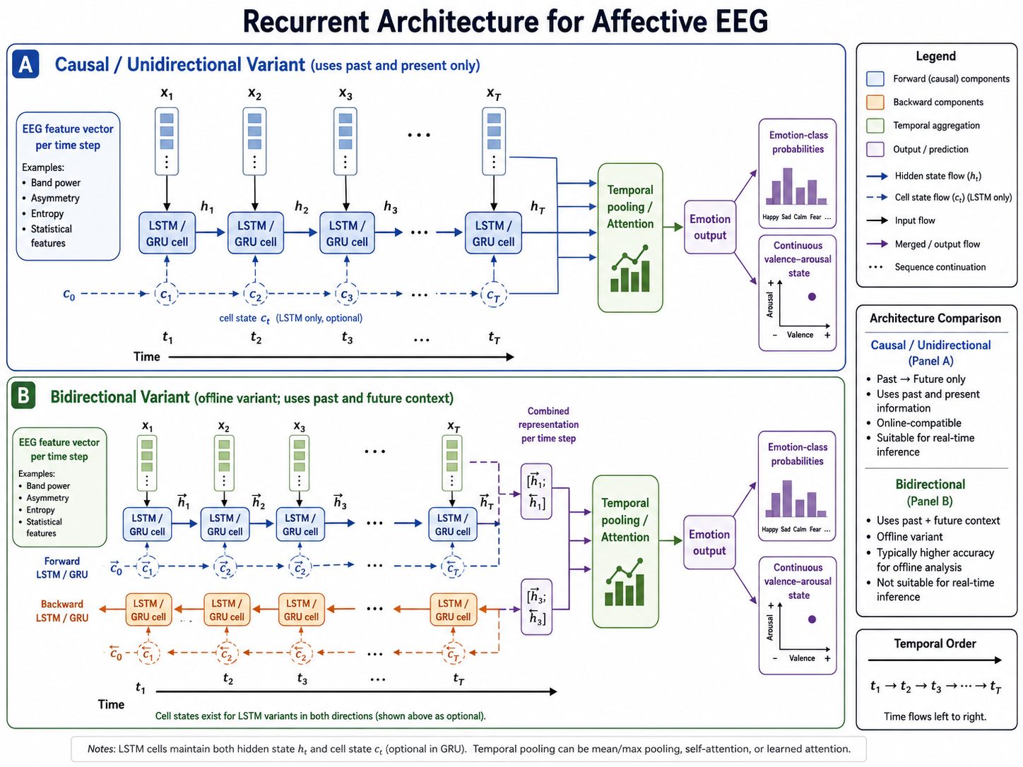
Figure 8.3: Recurrent architecture for affective EEG. LSTM or GRU cells propagate a learned hidden state through EEG time steps to represent temporal affect dynamics.
Theoretical Foundations
Vanilla RNN
A basic RNN updates hidden state sequentially:
Where:
- = hidden state at time
- = input at time
- matrices = weight matrices (shared across time steps)
- = output at time
Key insight: Same parameters applied to each time step (weight sharing), allowing variable-length sequences.
The Vanishing Gradient Problem
During backpropagation through time (BPTT), gradients multiply across time steps:
If products are < 1, gradients vanish (can't learn long dependencies). If products are > 1, gradients explode.
This limitation explains why a vanilla RNN can react well to the most recent EEG samples yet fail to connect an earlier rhythm or event with a later affective response. The goal of gated variants is not simply to add parameters; it is to create paths through time along which useful information and gradients can persist, while allowing irrelevant fluctuations to be forgotten.
Long Short-Term Memory (LSTM)
LSTMs solve this with memory cells and gating mechanisms:
Cell State : Stores long-term information
Gates: (Forget gate) (Input gate) (Cell candidate) (Output gate)
Updates:
The cell state acts as a "highway" for information, enabling long-range dependencies.
Gated Recurrent Unit (GRU)
A simpler variant with similar benefits:
(Reset gate) (Update gate)
Difference from LSTM:
- Fewer parameters (simpler, trains faster)
- Often comparable performance
- Good for smaller datasets
RNN Variants and Design Choices
The RNN family evolved to address the tension between temporal memory and practical training. A vanilla RNN is the simplest sequential baseline, but its hidden state can lose information over long recordings. LSTM adds a separate memory cell and explicit gates to preserve or discard information over time. GRU merges some of those gates into a lighter design, reducing parameters and training cost. Bidirectional RNNs process a complete sequence in both directions when future context is available, while attention-enhanced RNNs let the model emphasize a small number of informative moments instead of relying solely on the final hidden state.
For EEG, select the variant based on what is known when a prediction is needed. GRU is a sensible starting point for modest datasets or real-time systems; LSTM is useful when longer temporal context may matter; bidirectional models are suitable for offline analysis but cannot be used causally; and attention is helpful when emotion-relevant events are sparse. More elaborate variants do not automatically improve performance—limited subject diversity and inconsistent sequence definitions are often the larger bottlenecks.
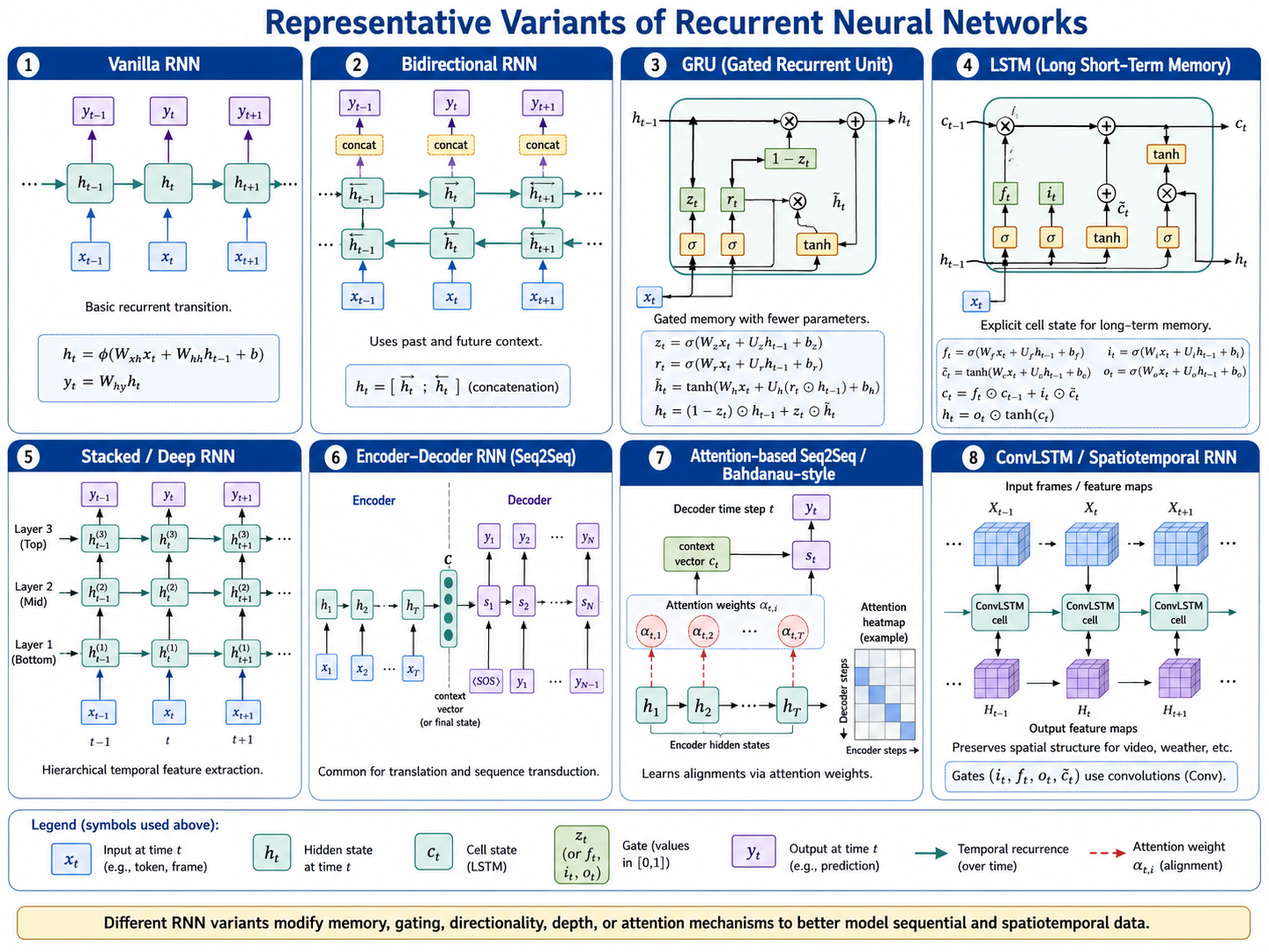
Figure 8.3b: RNN variants and their design motivations. Vanilla RNNs provide a simple recurrent baseline; LSTMs use gated memory cells to retain long-range information; GRUs achieve similar control with fewer parameters; bidirectional variants use both past and future context; and attention-enhanced variants focus the readout on the most informative time steps.
Adaptation to EEG-based Affective Computing
Why RNNs/LSTMs for EEG?
Advantages:
- Variable-length sequences: Handle sessions of different durations
- Long-term dependencies: Capture emotional state evolution over minutes
- Sequential reasoning: Model emotion dynamics explicitly
- Online prediction: Predict emotion at each time step if desired
Limitations:
- Computationally expensive (sequential processing, no parallelization)
- Require more data than CNNs
- Harder to interpret than CNNs
- May overfit on small datasets
- Training slower than CNNs
Typical Pipeline
The pipeline turns a continuous physiological recording into a sequence of model inputs. Its central modeling choice is the time scale of one recurrent step: individual samples preserve fine timing but create very long sequences, whereas window-level features reduce computation and may align better with slowly changing affect. Set the step size and sequence length from the expected duration of the target phenomenon, then keep that definition consistent across subjects and splits.
Raw EEG → Preprocessing → Segmentation → Sequences → LSTM → Emotion State
           (Filtering)     (Sliding        (Feed time   (Valence/
                            windows)       steps one by  Arousal)
                                          one)
Suitable Input Features
Representation Options
There is no universally best input representation. Direct time series retain waveform-level information but place the burden of feature extraction on the RNN. Band-filtered or engineered features inject domain knowledge and shorten the effective sequence, but can hide information that was not anticipated during feature design. Start with the simplest representation that matches the research question, and compare alternatives under the same subject-wise evaluation split.
Option 1: Multivariate Time Series
Direct input of multichannel EEG:
# Shape: (sequence_length, n_channels)
# Example: (2048, 14)  # 2048 time steps, 14 channels
# At 256 Hz, represents ~8 seconds of data

# LSTM processes:
# t=0: x[0, :] (first sample across 14 channels)
# t=1: x[1, :] (second sample across 14 channels)
# ...
# t=2047: x[2047, :] (last sample)
Advantages:
- Keeps spatial information (channel relationships)
- LSTM learns which channels are informative
- Natural representation
Disadvantages:
- Long sequences (high computational cost)
- May amplify noise
Option 2: Frequency-Filtered Channels
# Pre-filter into frequency bands
# Shape: (sequence_length, n_channels × n_bands)
# Example: (2048, 14 × 5) = (2048, 70)
# 5 bands: Delta, Theta, Alpha, Beta, Gamma per channel

# Reduces noise while preserving frequency information
# LSTM focuses on learning which frequencies matter
Option 3: Reduced Representation (Features × Time)
# Pre-extract features at each time step
# Shape: (sequence_length, n_features)
# Example: (1024, 128)

# Features computed in sliding windows:
# - PSD in each band
# - Statistical measures
# - Cross-frequency coupling

# Reduces computation but loses some information
Option 4: Spectral Features with Time Axis
# Short-time Fourier transform (STFT) per channel
# Shape: (sequence_length, n_frequencies)
# Time steps = frequency-time windows

# Example:
# - STFT window = 256 samples (1 sec at 256 Hz)
# - Hop = 64 samples (75% overlap)
# - 300 second session → ~1200 time steps
# - 257 frequency bins
Preprocessing for RNNs/LSTMs
RNNs repeatedly reuse their hidden state, so amplitude drift, artifacts, and inconsistent scaling can persist through many steps rather than remaining local errors. Filtering and normalization should therefore be fitted on training data only, while segmentation should avoid putting overlapping windows from the same recording into different splits. Otherwise, the model can appear to learn temporal affect dynamics while actually recognizing recording-specific leakage.
1. Signal Filtering
# Remove artifacts and noise
signal = bandpass_filter(signal, 0.5, 40)  # Hz
2. Normalization
# LSTM is sensitive to scale
# Per-channel z-score normalization:
for ch in range(n_channels):
    signal[ch] = (signal[ch] - signal[ch].mean()) / signal[ch].std()

# Or global normalization:
signal = (signal - signal.mean()) / signal.std()
3. Segmentation into Sequences
# For session-level emotion prediction:
session_signal = load_session()  # Entire emotional video

# Optional: Chunk into shorter sequences for more samples
# Long sequences (60 sec = 15360 samples at 256 Hz) may be
# too computationally expensive

chunk_size = 2048  # ~8 seconds
overlap = 0.5
chunks = chunk_signal(session_signal, chunk_size, overlap)
4. Optional Feature Extraction
# If using reduced representation, extract features per chunk:
features_per_chunk = []
for chunk in chunks:
    psd = compute_psd(chunk)
    stats = compute_statistics(chunk)
    features = np.concatenate([psd, stats])
    features_per_chunk.append(features)
Network Architecture for EEG
The architecture variants below change how much context the recurrent representation can retain and how it is summarized. A single recurrent layer is a transparent baseline; stacking increases abstraction but can make optimization harder; bidirectionality trades real-time use for access to future context; and attention addresses the “last-state bottleneck” by allowing the classifier to inspect multiple time steps. Compare each added mechanism against a simpler baseline before attributing an improvement to temporal reasoning.
Simple LSTM (Single Layer)
Input: (sequence_length, n_channels)
Example: (2048, 14)
   ↓
LSTM(128 units)  [processes each time step sequentially]
   ↓
Dense(64) → ReLU
   ↓
Output (emotion class)
Use when: Limited data or computational resources.
Implementation:
model = Sequential([
    LSTM(128, input_shape=(2048, 14)),
    Dense(64, activation='relu'),
    Dropout(0.5),
    Dense(num_emotions, activation='softmax')
])
Stacked LSTM (Multiple Layers)
Input: (sequence_length, n_channels)
Example: (2048, 14)
   ↓
LSTM(128, return_sequences=True)  [output shape: (2048, 128)]
   ↓
LSTM(64, return_sequences=True)   [output shape: (2048, 64)]
   ↓
LSTM(32)                           [output shape: (32,)]
   ↓
Dense(64) → ReLU → Dropout(0.5)
   ↓
Output (emotion class)
Why stack layers: Each layer learns higher-level temporal patterns.
Key parameter: return_sequences=True passes full sequence to next layer.
Bidirectional LSTM
Input: (sequence_length, n_channels)
   ↓
Forward LSTM  (→)  →
                    ↓ Concatenate
Backward LSTM (←)  ←
   ↓
Combined output: (sequence_length, 2 × units)
   ↓
Dense layers
   ↓
Output
Advantage: Context from both past and future time steps.
Disadvantage: Not suitable for real-time prediction (needs future data).
Attention-Enhanced LSTM
Input: (sequence_length, n_channels)
   ↓
LSTM(128, return_sequences=True)  [(T, 128)]
   ↓
Attention mechanism
  - Computes importance weights for each time step
  - Produces weighted context
   ↓
Context vector
   ↓
Dense layers
   ↓
Output
Benefit: Focus on important time periods (e.g., video peaks).
LSTM for Sequence-to-Sequence Prediction
For predicting emotion at each time step:
Input: (sequence_length, n_channels)
   ↓
LSTM(128, return_sequences=True)  [(T, 128)]
   ↓
Time-distributed Dense(64)       [(T, 64)]
   ↓
Time-distributed Output          [(T, num_emotions)]
   ↓
Output shape: one prediction per time step
Implementation Considerations
Implementation details often determine whether an RNN learns temporal structure or merely overfits sequence length and subject identity. The following choices are connected: longer sequences increase contextual coverage but strain memory and gradients; batching requires padding or packing variable-length sessions correctly; and regularization must not erase the small changes that carry affective information. Monitor validation performance by subject and inspect performance across sequence lengths rather than choosing settings solely from training loss.
Sequence Length Selection
Trade-off between temporal context and computational cost:
| Sequence Length | Duration (at 256 Hz) | Computational Cost | Temporal Context |
|---|---|---|---|
| 512 | 2 sec | Low | Very local |
| 1024 | 4 sec | Low-Medium | Local |
| 2048 | 8 sec | Medium | Medium |
| 4096 | 16 sec | Medium-High | Good |
| 8192 | 32 sec | High | Excellent |
Guideline: Start with 2048-4096 (8-16 seconds), then adjust based on:
- Emotional phenomena duration (typically 4-60 seconds)
- Available computational resources
- Dataset size (longer sequences → fewer training samples)
Batch Size and Sequence Processing
LSTM processes sequences in batches:
# Batch shape: (batch_size, sequence_length, n_features)
# Example: (32, 2048, 14)
# - 32 sequences
# - Each 2048 time steps
# - Each time step has 14 channel values

model.fit(X, y, batch_size=32, epochs=100)
Memory consideration:
Memory = batch_size × sequence_length × n_features × 4 bytes
Example: 32 × 2048 × 14 × 4 = ~3.6 MB per batch
Gradient Issues and Solutions
Vanishing/Exploding Gradients (even with LSTM):
Gradient clipping: Limit gradient magnitude
optimizer = Adam(clipvalue=1.0) # Clip to ±1.0Layer normalization: Normalize hidden state
from tensorflow.keras.layers import LSTM, LayerNormalization
LSTM(128)
LayerNormalization()
Residual connections: Skip connections for deeper networks
# Output of layer i + input to layer i
Dropout in RNNs
Standard dropout can be problematic. Use recurrent dropout:
LSTM(128, dropout=0.3,           # Dropout on inputs
     recurrent_dropout=0.3)      # Dropout on recurrent connections
Example Application: Online Emotion Tracking
Online tracking highlights the distinction between causal and offline sequence models. At time $t$, the model may only use EEG observed up to $t$; bidirectional processing and future-window features would leak information that a deployed system cannot have. A useful evaluation should therefore simulate the streaming setting, report prediction latency, and assess whether outputs remain stable rather than fluctuating with every short-lived artifact.
Task
Predict valence/arousal continuously during video-induced emotion.
Architecture
from tensorflow.keras import Sequential
from tensorflow.keras.layers import LSTM, Dense, Dropout, Input

model = Sequential([
    Input(shape=(2048, 14)),  # 8-sec windows, 14 channels

    # LSTM layers
    LSTM(256, return_sequences=True, recurrent_dropout=0.2),
    Dropout(0.3),

    LSTM(128, return_sequences=True, recurrent_dropout=0.2),
    Dropout(0.3),

    LSTM(64),  # Final LSTM, returns single output
    Dropout(0.3),

    # Dense layers
    Dense(128, activation='relu'),
    Dropout(0.5),

    Dense(64, activation='relu'),
    Dropout(0.3),

    # Output: valence and arousal
    Dense(2, activation='linear')  # [valence ∈ [-1,1], arousal ∈ [0,1]]
])

model.compile(
    optimizer='adam',
    loss='mse',
    metrics=['mae']
)
Preprocessing
import numpy as np

# 1. Load EEG session
session = load_eeg_session()  # (14 channels, ~300 sec × 256 Hz)

# 2. Filter
session = bandpass_filter(session, 0.5, 40)

# 3. Create sliding windows
window_size = 2048
overlap = 0.5
step = int(window_size * (1 - overlap))
windows = []

for start in range(0, session.shape[1] - window_size, step):
    window = session[:, start:start+window_size].T  # (T, channels)
    windows.append(window)

windows = np.array(windows)

# 4. Normalize
windows_norm = (windows - windows.mean(axis=(0, 2))) / windows.std(axis=(0, 2))

# 5. Get labels
valence_labels = get_valence_labels()      # Continuous values
arousal_labels = get_arousal_labels()      # Continuous values
labels = np.stack([valence_labels, arousal_labels], axis=1)

# 6. Train
history = model.fit(
    windows_norm, labels,
    epochs=100,
    batch_size=32,
    validation_split=0.2
)
Advantages and Disadvantages
| Aspect | LSTM/RNN | CNN | MLP |
|---|---|---|---|
| Temporal modeling | Excellent (explicit) | Good (local) | Poor |
| Variable-length input | ✓ Yes | ✗ No | ✗ No |
| Computational efficiency | Low | High | Very High |
| Memory requirements | High | Medium | Low |
| Data requirements | High (1000+) | Medium (500+) | Low (100+) |
| Training speed | Slow | Fast | Very Fast |
| Inference speed | Slow | Fast | Very Fast |
| Interpretability | Low | Medium | High |
Comparison with CNNs for EEG
| Factor | CNN | LSTM |
|---|---|---|
| Local patterns | Excellent | Good |
| Long-range patterns | Implicit, limited | Explicit, excellent |
| Noise robustness | Good | Moderate |
| Fixed window modeling | Ideal | Overkill |
| Session-level modeling | Via aggregation | Natural |
| Real-time capability | Good | Fair |
| Training data needed | Medium | High |
When to Use RNNs/LSTMs
Choose RNNs/LSTMs when:
- Modeling entire emotional sessions (not just windows)
- Emotional state evolves over time
- Predicting emotion at each time point
- Variable-length sequences are natural
- Dataset is sufficiently large (1000+ samples)
- Computational resources available
Stick with CNNs when:
- Processing fixed-length windows
- Limited training data
- Real-time inference critical
- Computational resources limited
Use both (Hybrid) when:
- Large, diverse datasets
- Both local and global patterns matter
- Computational resources sufficient
Best Practices
- Start with moderate sequence length: 2048-4096 samples (8-16 sec)
- Use bidirectional LSTMs when future context is available
- Add layer normalization to stabilize training
- Use recurrent dropout instead of standard dropout
- Implement gradient clipping to handle exploding gradients
- Monitor for overfitting: Use validation data and early stopping
- Validate generalization: LOSO cross-validation across subjects
- Consider computational cost in deployment scenarios
Summary
RNNs and LSTMs excel at modeling temporal dynamics in EEG signals. They naturally handle variable-length sequences and can capture long-range emotional state evolution. However, they demand:
- More training data than simpler models
- Greater computational resources
- Longer training times
- Careful hyperparameter tuning
LSTMs are particularly valuable for:
- Session-level emotion analysis
- Online emotion prediction
- Capturing emotional dynamics over minutes
- Sequential decision-making tasks
For many EEG applications with fixed-window analysis and limited data, hybrid architectures (CNN + LSTM) often provide the best balance of performance and efficiency (see next sections).
Next: Transformer Models
References
- Elman, J. L. (1990). Finding structure in time. Cognitive Science, 14(2), 179–211.
- Hochreiter, S., and Schmidhuber, J. (1997). Long short-term memory. Neural Computation, 9(8), 1735–1780.
- Cho, K., van Merriënboer, B., Gulcehre, C., et al. (2014). Learning phrase representations using RNN encoder–decoder for statistical machine translation. In EMNLP.
- Pascanu, R., Mikolov, T., and Bengio, Y. (2013). On the difficulty of training recurrent neural networks. In ICML.
- Lipton, Z. C., Berkowitz, J., and Elkan, C. (2015). A critical review of recurrent neural networks for sequence learning. arXiv:1506.00019.