Causal Online Signal Processing and Inference

Causality is a constraint on information, not a synonym for "the code ran in a loop." At decision time $t$ , a causal feature, state estimate, or action may use only information that was available at or before $t$ . Availability includes samples, labels, calibration statistics, filter state, and model parameters. An operation that looks at a future sample, a later rating, or a statistic fitted on the whole recording is not causal at $t$ , even if it is later wrapped in a streaming API.

Chapter 4 distinguishes batch prediction, state tracking, and forecasting. Chapter 6 distinguishes offline and online preprocessing. This section specifies the runtime counterpart: how windows, state, and models must be implemented if those distinctions are to survive contact with a live stream.

Decision Time, Windows, and Cadence

Let $x(\tau)$ denote the EEG (and any auxiliary) sample whose availability time is $\tau$ . A causal estimator at decision time $t$ has the form

$\hat{s}_t = f\!\left(\{x(\tau):\tau \le t\},\; \theta_t,\; h_t\right),$

where $\theta_{t}$ are model and calibration parameters that themselves must have been determined without future data.

The carried state $h_{t}$ includes filter memory, recurrent hidden state, and running moments. In practice $f$ consumes a window of length $W$ ending at $t$ ,

$w_t = \{x(\tau): t-W < \tau \le t\},$

advanced with stride $\Delta$ . The lookback horizon is $W$ . The decision cadence is $1/\Delta$ if the pipeline meets its deadline. Overlap $W-\Delta$ increases update rate and temporal correlation; it does not grant access to the future.

Three tasks must not be collapsed:

Task	Target	Information cutoff	Typical failure if confused
Event detection	Whether an event has already begun	Evidence up to $t$	Using post-event samples to "detect" onset
Current-state estimation	$\hat{s}_t$ at time $t$	$\tau \le t$	Centered windows that straddle $t$
Forecasting	$\hat{s}_{t+\delta}$ for horizon $\delta>0$	$\tau \le t$	Reporting a forecast as a present-state reading

Label time is a separate axis. The time a label describes is not the time the label becomes available. A continuous rating issued at 12.8 s about affect at 12.5 s is not supervision for a decision at 12.5 s. A trial-level rating collected after the clip ends is not a window-level target for any moment during the clip; it is bag-level supervision, as discussed in Chapter 11. Online training or evaluation that copies a future summary onto past windows is a supervision mismatch, not a streaming implementation detail.

State, Warm-Up, and Boundaries

Online filters and recurrent models are stateful. An IIR high-pass filter carries internal delay-line values. An LSTM carries a hidden state. Incremental spectral estimates carry running sums. That state is legitimate causal context if it was produced only from $\tau \le t$ . It is leakage if it was initialized from a future epoch, from a whole-recording mean, or from a bidirectional pass.

Warm-up is the interval during which state is not yet representative: filter transients, unfilled windows, unset running statistics. Decisions issued during warm-up should be excluded from scored evaluation or explicitly marked as initializing. Boundary behavior at session start, after a dropout, and after a device reconnect must be declared. The honest options are to reset state, to restore a serialized state from a previous epoch of the same session, or to remain in a degraded mode until a new warm-up completes. There is no third option in which the model "just continues" across a discontinuity without a policy.

Online Normalization and Causal Filtering

Normalization is a common source of future-information leakage. Whole-recording z-scoring, full-trial baselines, and any statistic that uses validation or test samples are offline operations. Online alternatives include:

statistics frozen from a calibration period that ended before scoring begins;
causal running means and variances with an explicit update rule and a declared half-life;
session-level statistics computed only from data already observed in that session, never from later minutes.

Widmann, Schröger, and Maess emphasize that filter choice is a causal design decision, not only a frequency-domain convenience. Zero-phase (forward–backward) filtering uses the future of the block. Centered moving-average smoothers do the same. Full-trial ICA, bidirectional recurrent or Transformer encoders, and any smoother whose kernel has support after $t$ are similarly noncausal at $t$ . They remain useful for offline analysis. They do not support a current-time real-time claim.

Causal counterparts exist. A forward-only IIR or minimum-phase FIR filter uses only past and present samples; it imposes group delay that must enter $L_{\mathrm{preprocessing}}$ . Unidirectional recurrent models can run sample-by-sample or window-by-window with carried state. Causal attention can restrict keys and values to $\tau \le t$ . Incremental feature computation (running power, exponentially weighted covariance, sliding STFT with a causal hop) avoids recomputing a whole trial and makes the cost of each update closer to the cost that will be paid at runtime.

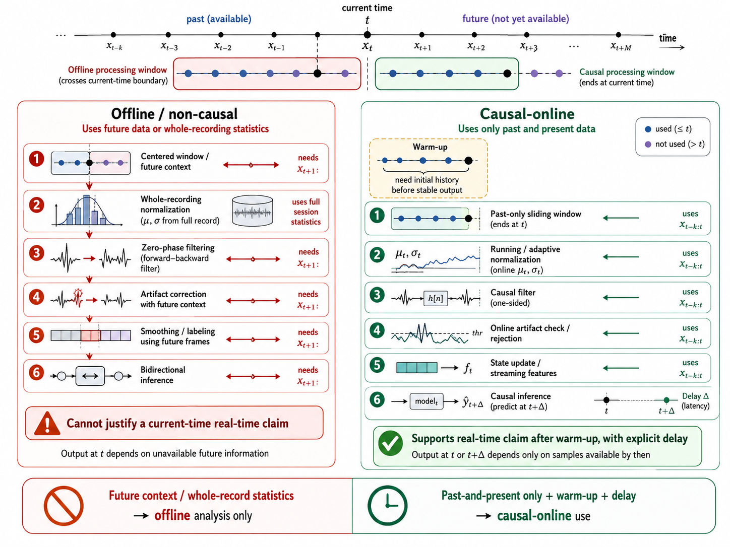
Figure 10.2: Offline versus causal-online information availability. Centered filters, future context windows, whole-recording normalization, and bidirectional models invalidate a current-time claim. Causal filters, past-only windows, frozen or running statistics, and unidirectional state are the corresponding online tools.

Offline operation	Why it leaks at time $t$	Causal online counterpart
Zero-phase / `filtfilt`	Uses future samples in the reverse pass	Forward IIR or causal FIR, with declared group delay
Centered smoother	Kernel extends after $t$	Causal exponential or one-sided moving average
Whole-recording z-score	Uses future minutes of the session	Frozen calibration stats or causal running moments
Full-trial baseline	Subtracts a statistic that includes post- $t$ data	Pre-window or running baseline ending at $t$
Bidirectional LSTM / Transformer	Backward states depend on the future	Unidirectional or causally masked model
ICA fitted on the whole recording	Mixing matrix sees the entire session	Frozen unmixing from calibration, or online artifact rules
Test-set or full-dataset scaling	Uses held-out distribution	Training- or calibration-only transforms

Resources and Batch-Size-One Inference

A real-time model runs under CPU or GPU load, memory limits, battery and thermal constraints, and often a shared operating system. Compression, quantization, distillation, and smaller architectures are engineering responses to those limits, not automatic accuracy improvements. The relevant measurement is latency and jitter at batch size one on the target device, with the rest of the pipeline running. Offline throughput on a GPU with batch 64 does not establish real-time performance. A model that is fast on average but stalls at the 99th percentile when the garbage collector or a display compositor runs is not meeting its latency budget.

A Timestamp-Aware Inference Loop

The following sketch is technically coherent. It is not a drop-in driver for every headset.

# Illustrative causal loop. Device APIs, clock domains, and
# model interfaces differ; this is not a complete implementation.

for packet in inlet:
    t_arr = now()
    for sample in packet.samples:
        if not continuity_ok(buffer, sample.t_dev):
            quality.mark_gap(sample.t_dev)
            state.reset_or_hold()
            policy.enter("DEGRADED")
            log.lineage(sample, quality, None, "gap")
            continue

        buffer.push(sample)  # ring buffer indexed by t_dev
        quality.update(sample, buffer)

        if not buffer.has_causal_window(W, t_end=sample.t_dev):
            continue  # warm-up: window not yet full

        window = buffer.causal_window(W, t_end=sample.t_dev)
        if quality.untrustworthy(window):
            policy.enter("ABSTAIN")
            act = policy.safe_action()
            log.lineage(window, quality, None, act)
            emit(act)
            continue

        x, state = preprocess_causal(window, state)   # filter state
        y_hat, u_hat = model.infer(x, state.h)        # prediction, uncertainty
        decision = policy.decide(y_hat, u_hat, quality, t=sample.t_dev)

        if decision.kind in ("ACT", "ABSTAIN", "SAFE_FALLBACK"):
            emit(decision.action)
        log.lineage(
            t_dev=sample.t_dev, t_arr=t_arr, t_dec=now(),
            quality=quality.snapshot(), y_hat=y_hat, u_hat=u_hat,
            state=policy.mode, action=decision, versions=versions,
        )

The important properties are chronological consumption, a timestamped buffer, an explicit continuity check, a causal window, stateful preprocessing, a separate uncertainty estimate, a policy that may refuse to act, and a lineage record that can replay the decision.

Practical Recommendations

Write the information cutoff next to every transform: which timestamps it may read.
Treat filter state, recurrent state, and running statistics as versioned objects with reset rules.
Exclude warm-up from scored metrics or report it separately.
Measure inference at batch size one on the deployment device, under representative load.
If a bidirectional or zero-phase method is used, describe the system as offline or near-causal with a stated noncausal span, not as real-time current-state estimation.

Next: Robust Operation, Adaptation, and Safe Control

References

Widmann, A., Schroger, E., and Maess, B. (2015). Digital filter design for electrophysiological data: A practical approach. Journal of Neuroscience Methods, 250, 34-46.
Lotte, F., Bougrain, L., Cichocki, A., Clerc, M., Congedo, M., Rakotomamonjy, A., and Yger, F. (2018). A review of classification algorithms for EEG-based brain-computer interfaces: a 10 year update. Journal of Neural Engineering, 15(3), 031005.
Wolpaw, J. R., and Wolpaw, E. W. (Eds.). (2012). Brain-Computer Interfaces: Principles and Practice. Oxford University Press.
Schalk, G., McFarland, D. J., Hinterberger, T., Birbaumer, N., and Wolpaw, J. R. (2004). BCI2000: A general-purpose brain-computer interface (BCI) system. IEEE Transactions on Biomedical Engineering, 51(6), 1034-1043.

10.2 Causal Online Signal Processing and Inference