Trending Architectures for EEG-based Affective Computing
Overview
The landscape of deep learning is evolving rapidly. Beyond the established architectures (MLP, CNN, RNN, Transformer, GNN), a new wave of models is emerging with fundamentally different design principles. This section surveys trending architectures that are beginning to impact EEG-based affective computing, discussing their theoretical motivation, practical potential, and current limitations.
Kolmogorov-Arnold Networks (KANs)
Motivation
Traditional MLPs use fixed activation functions (e.g., ReLU, sigmoid) on nodes and learn only the linear weights between layers. KANs invert this paradigm: they use learnable activation functions on edges while nodes perform simple summation.
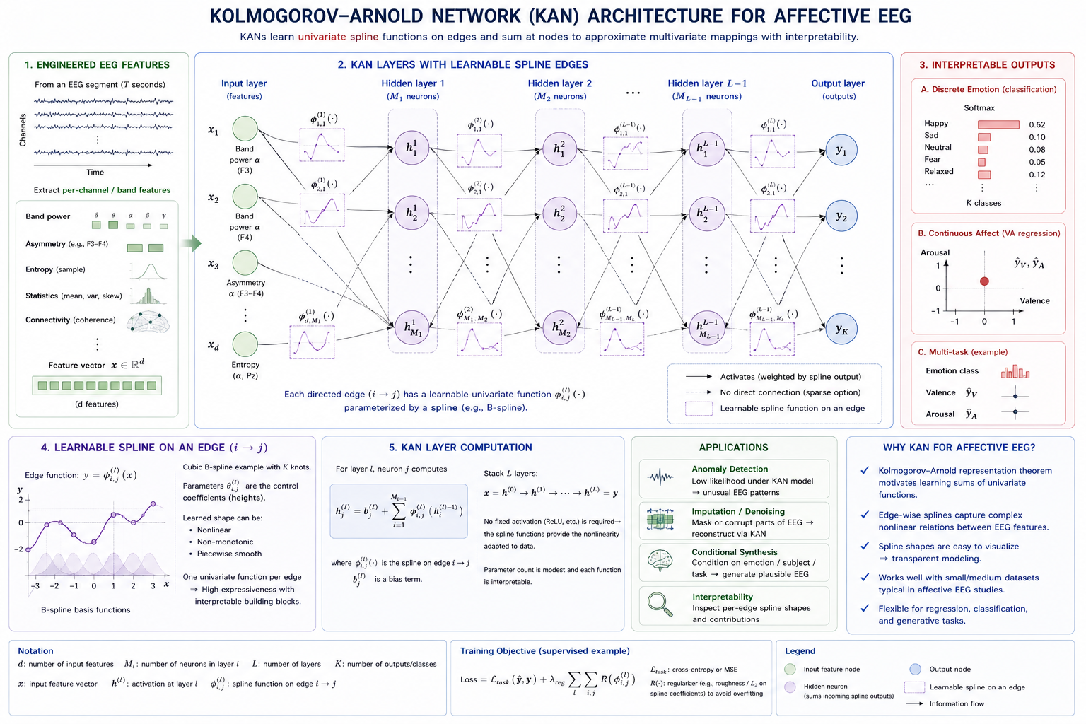
Figure 8.10: KAN architecture for affective EEG. KANs replace fixed activations on nodes with learnable spline functions on edges, yielding compact, interpretable feature models for affective EEG.
Theoretical Foundation
Based on the Kolmogorov-Arnold representation theorem:
Any multivariate continuous function can be represented as:
where and are univariate continuous functions.
A KAN layer replaces the linear weight with a learnable univariate function :
MLP:
KAN:
where each is a learnable spline function.
Learnable Activation Functions
KANs typically parameterize using B-splines:
where:
- are B-spline basis functions
- are learnable coefficients
- control the mix of base activation and spline component
- is the base activation
Key Properties
| Property | MLP | KAN |
|---|---|---|
| Learnable parameters | Weights on connections | Activation functions on edges |
| Expressiveness | Good with large width | Good with small width |
| Interpretability | Low (black box) | Higher (spline visualization) |
| Scaling law | Power law in parameters | Faster scaling (fewer params) |
| Training speed | Fast | Currently slower (10×) |
| Symbolic regression | Difficult | Natural fit |
Adaptation to EEG Affective Computing
Potential advantages:
- Interpretability: Visualize which input features → which frequencies are learned as activation patterns
- Parameter efficiency: Small KAN may match larger MLP on limited EEG data
- Feature discovery: Splines can naturally represent frequency-selective responses (matches how brain processes rhythms)
- Symbolic insight: May extract human-readable rules about EEG-emotion relationships
Current challenges:
- Training speed (active research area)
- Limited tooling (no stable Keras/PyTorch ecosystem yet)
- Validation on real EEG tasks is nascent
- Batch size / GPU optimization not mature
Suitable Input Features
KANs work best with pre-extracted features (similar to MLPs):
- Frequency band powers (5 bands × 14 channels = 70 features)
- Frontal asymmetry indices
- Statistical moments (mean, variance, skewness, kurtosis)
- Entropy measures
The small number of features per input makes KANs tractable and the spline activations can discover non-linear feature interactions.
Conceptual Architecture
Input: (128 hand-crafted features)
   ↓
KAN Layer 1: 128 inputs → 64 outputs
  - 128×64 = 8192 learnable spline functions φᵢⱼ(x)
  - Each φ: B-spline of order k=3, G=5 grid points
   ↓
KAN Layer 2: 64 → 32
  - 64×32 = 2048 learnable splines
   ↓
KAN Layer 3: 32 → 3 (emotion classes)
  - 32×3 = 96 learnable splines
   ↓
Output: softmax over 3 classes
Total parameters: ~10,336 spline functions (each with ~8 coefficients) ≈ 82K params Equivalent MLP: Would need similar or more parameters for comparable expressiveness.
Symbolic Regression for EEG Biomarkers
A unique KAN capability: after training, simplify the learned splines to symbolic formulas:
# After training KAN on EEG → emotion:
# φ₁(x) learned: 0.3·x² - 0.1·x + 0.5
# φ₂(x) learned: sin(2π·0.5·x)  (frequency detector!)
# φ₃(x) learned: e^(-|x|)

# Prune and symbolic-ify:
# emotion_score ≈ 0.3·(alpha_power)² - 0.1·(theta/beta ratio)
#                     + sin(2π·0.5·frontal_asymmetry)
This could discover interpretable EEG biomarkers for emotions — a holy grail in affective neuroscience.
Current Limitations for EEG
- No temporal modeling: KAN is a static function approximator; needs coupling with temporal architectures
- Experimental codebase:
pykanlibrary is research-grade - Scalability: Current implementations struggle with >100 input features
- Few EEG benchmarks: Waiting for community validation
State Space Models (SSMs) and Mamba
Motivation
Transformers have attention complexity. State Space Models offer sequence modeling with competitive performance — a game-changer for long EEG recordings.
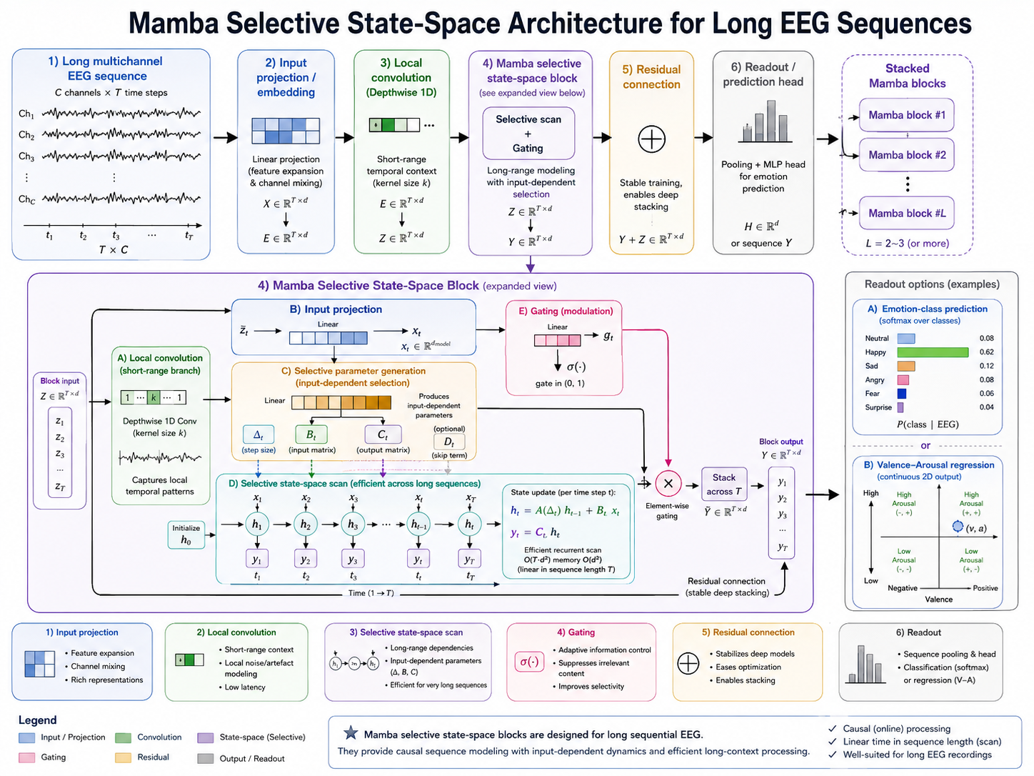
Figure 8.11: Mamba selective state-space architecture for affective EEG. Selective state-space models provide linear-scaling sequence processing for long EEG recordings.
Theoretical Foundation
A continuous-time SSM maps a 1D input to output through a latent state :
Discretized with step size :
where , .
Mamba: Selective SSM
Key innovation: Make SSM parameters input-dependent (selective):
This allows the model to:
- Selectively remember or ignore information based on input
- Focus on emotionally relevant EEG segments
- Adapt filtering behavior to signal content
Mamba Architecture Block
Input: (T, d)  # T time steps, d channels
   ↓
Linear projection → (T, 2d)
   ↓
1D Convolution (local mixing)
   ↓
SiLU activation
   ↓
Selective SSM (Mamba core)
  - Δ = softplus(Linear(x) + bias)
  - B = Linear(x)
  - C = Linear(x)
  - Discretize A with Δ
  - Parallel scan: xₖ = Āₖxₖ₋₁ + B̄ₖuₖ
   ↓
SiLU gating (elementwise with residual)
   ↓
Linear projection → (T, d)
   ↓
+ Residual connection
Adaptation to EEG Affective Computing
Key advantages for EEG:
- Linear scaling: complexity enables processing entire sessions (30+ minutes at 256 Hz ≈ 460,000 samples)
- Selectivity: Mamba learns to attend to emotionally salient segments (e.g., video climax)
- Continuous-time heritage: SSMs naturally model continuous physiological signals
- Efficient inference: Fast autoregressive generation for real-time emotion tracking
- Long-range dependencies: No attention bottleneck; captures slow emotional drifts
Comparison with Transformers for EEG:
| Aspect | Transformer | Mamba/SSM |
|---|---|---|
| Complexity | ||
| Max practical length | ~4,096 samples | >100,000 samples |
| Memory usage | Quadratic | Linear |
| Training speed | Fast (parallel) | Fast (parallel scan) |
| Long-range modeling | Excellent (global attention) | Excellent (selective memory) |
| Interpretability | Attention maps | Less interpretable |
| Maturity for EEG | Established | Emerging |
Suitable Input Features
Raw multichannel EEG (ideal for Mamba):
# Shape: (batch, T, channels)
# T = 30 seconds × 256 Hz = 7,680  (easily handled)
# T = 5 minutes × 256 Hz = 76,800  (difficult for Transformer, fine for Mamba)
Preprocessed features:
# Per-time-step spectral features
# Shape: (batch, T, n_bands × n_channels)
# T = 120 time windows (2 sec each for 4 min session)
Multi-scale SSM:
# Process EEG at multiple temporal resolutions
# Fast stream: 256 Hz raw
# Slow stream: Downsampled envelope
# → Multiple parallel SSM branches
Conceptual Mamba Model for EEG Emotion Recognition
# Note: This uses the mamba-ssm library (research code)
# pip install mamba-ssm (requires CUDA)

import torch
import torch.nn as nn
from mamba_ssm import Mamba

class EEGMamba(nn.Module):
    def __init__(self, n_channels=14, d_model=256, n_layers=4, n_emotions=3):
        super().__init__()

        # Project EEG channels to model dimension
        self.input_proj = nn.Linear(n_channels, d_model)

        # Stack of Mamba blocks
        self.mamba_blocks = nn.ModuleList([
            MambaBlock(d_model) for _ in range(n_layers)
        ])

        # Layer norm
        self.norm = nn.LayerNorm(d_model)

        # Classification head
        self.classifier = nn.Sequential(
            nn.Linear(d_model, 128),
            nn.ReLU(),
            nn.Dropout(0.3),
            nn.Linear(128, n_emotions)
        )

    def forward(self, x):
        """
        x: (batch, T, n_channels) - e.g., (32, 7680, 14)
        """
        x = self.input_proj(x)  # (B, T, d_model)

        for block in self.mamba_blocks:
            x = block(x)  # (B, T, d_model)

        x = self.norm(x)

        # Pool across time (mean of last 25% to focus on final state)
        T = x.shape[1]
        x = x[:, -T//4:, :].mean(dim=1)  # (B, d_model)

        return self.classifier(x)

class MambaBlock(nn.Module):
    def __init__(self, d_model):
        super().__init__()
        self.mamba = Mamba(
            d_model=d_model,
            d_state=16,      # SSM state dimension
            d_conv=4,        # Conv kernel size
            expand=2,        # Expansion factor
        )
        self.norm = nn.LayerNorm(d_model)

    def forward(self, x):
        return x + self.mamba(self.norm(x))
Preprocessing Considerations
# Mamba processes raw sequences → minimal preprocessing needed

# 1. Bandpass filter to remove DC drift and high-freq noise
signal = bandpass_filter(signal, 0.5, 40)

# 2. Per-channel normalization
for ch in range(n_channels):
    signal[ch] = (signal[ch] - signal[ch].mean()) / (signal[ch].std() + 1e-6)

# 3. No segmentation needed! Mamba handles long sequences
#    Optionally chunk for more training samples
#    session_signal shape: (T_total, n_channels)

# 4. Create sliding windows for training:
#    window_size = 7680  # 30 seconds at 256 Hz
#    stride = 3840        # 50% overlap
Current Status
- Mamba-1 (Dec 2023): Introduced selective SSM, matched Transformers on language
- Mamba-2 (May 2024): Connection to attention, faster training, SSD framework
- EEG applications: Early papers showing competitive/better results than Transformer-LSTM hybrids
- Limitations: GPU-optimized (CUDA required), research ecosystem developing
Spiking Neural Networks (SNNs)
Motivation
The brain communicates via spikes, not continuous values. SNNs are neuromorphic — they process information as discrete spike events, making them the most biologically plausible architecture and extremely energy-efficient.
Key Concepts
Leaky Integrate-and-Fire (LIF) neuron:
When membrane potential reaches threshold :
- Neuron fires a spike
- resets to
- Refractory period begins
Spike encoding:
# Rate coding: firing rate ∝ signal amplitude
# Temporal coding: spike timing carries information
# Population coding: groups of neurons encode features
Adaptation to EEG
Why SNNs fit EEG:
- Brain signals are fundamentally spiking → natural match
- Ultra-low power: suitable for wearable EEG emotion monitoring
- Temporal precision: millisecond-scale dynamics match EEG resolution
- Event-driven processing: only compute when spikes occur (sparse computation)
- Online learning: Can adapt continuously during use
Spike encoding strategies for EEG:
Rate coding: EEG amplitude → firing rate
spike_rate = (signal - min_threshold) / (max_threshold - min_threshold) * max_rateDelta modulation: Spike when signal changes significantly
spike[t] = 1 if |signal[t] - signal[t-1]| > threshold else 0Phase coding: Spike at specific phases of oscillatory activity
# Spike at alpha/theta phase peaks
spike[t] = 1 if phase[t] ≈ target_phase else 0
SNN Architecture for EEG Emotion
EEG → Spike Encoder → SNN Layers → Readout → Emotion
│                        │
│  Rate/Temporal/       │  LIF neurons
│  Phase encoding       │  Synaptic plasticity
│                        │  Sparse activity
Energy Efficiency Comparison
| Architecture | Operations/sample | Relative Energy | Hardware |
|---|---|---|---|
| CNN | ~10M FLOPs | 1× | GPU/CPU |
| LSTM | ~50M FLOPs | 5× | GPU/CPU |
| Transformer | ~100M FLOPs | 10× | GPU |
| SNN (neuromorphic) | ~0.1M spikes | 0.01× | Neuromorphic chip |
This makes SNNs compelling for wearable EEG devices that need real-time, all-day emotion monitoring.
Current Limitations
- Training difficulty: Non-differentiable spikes → surrogate gradients needed
- Software ecosystem: Less mature than standard deep learning frameworks
- Accuracy gap: Often slightly below equivalent ANNs on complex tasks
- Hardware dependency: Full efficiency only on neuromorphic chips (Loihi, TrueNorth)
- Limited pre-training: No large-scale SNN pre-trained models for EEG
Foundation Models and Large EEG Models
Motivation
In NLP and vision, scaling laws have shown that larger models trained on massive data consistently improve. The EEG community is beginning to explore this paradigm.
Key Approaches
EEG Pre-training Objectives
Masked Signal Modeling (analogous to BERT):
Mask random time segments → predict masked EEG
→ Model learns general EEG representations
Contrastive Learning (SimCLR-style):
Augment EEG segment → encode → maximize similarity with original
→ Model learns invariant representations
Next-Segment Prediction:
Given EEG[t], predict EEG[t+1]
→ Model learns temporal dynamics
Cross-Modal Alignment:
Align EEG with emotion labels, video features, or physiological signals
→ Multi-modal foundation
Architecture
[Massive Pre-training on 100K+ hours of EEG]
        ↓
Pre-trained EEG Encoder (Transformer/Mamba)
        ↓
[Fine-tune on specific task with small labeled data]
        ↓
Emotion Recognition | Stress Detection | Fatigue Monitoring
EEG-Specific Challenges
| Challenge | NLP/Vision | EEG |
|---|---|---|
| Data volume | Billions of samples | Typically <1000 sessions |
| Standardization | Standard tokenizers/resolutions | Varying electrode counts, sampling rates |
| Labels | Abundant | Sparse, subjective |
| Domain shift | Moderate | Severe (across subjects/devices) |
| Privacy | Manageable | Highly sensitive (brain data) |
Notable Initiatives
- BIOT (Biosignal Transformer): Pre-training on multiple biosignal datasets
- EEGNet pre-training: Transfer from large motor imagery datasets
- BENDR (BErt-like EEG Representations): Masked modeling on Temple University EEG corpus
- LaBraM (Large Brain Model): Pre-training on multi-center EEG data
Adaptation to Affective Computing
# Example workflow:
# 1. Load pre-trained EEG foundation model
encoder = load_pretrained_eeg_model('biot-base')

# 2. Freeze most layers
for param in encoder.parameters():
    param.requires_grad = False

# 3. Add emotion classification head
classifier = nn.Sequential(
    nn.Linear(encoder.hidden_dim, 128),
    nn.ReLU(),
    nn.Linear(128, 3)  # valence classes
)

# 4. Fine-tune on small affective EEG dataset
fine_tune(encoder, classifier, emotion_dataset)
Neural Ordinary Differential Equations (Neural ODEs)
Motivation
Standard neural networks have discrete layers. Neural ODEs model continuous depth, treating network depth as a continuous variable — ideal for continuous-time signals like EEG.
Formulation
A residual network layer:
A Neural ODE takes the limit as step size → 0:
The output is obtained by solving this ODE:
Advantages for EEG
- Continuous time: Natural for analog EEG signals
- Adaptive computation: ODE solver adjusts step size based on signal complexity
- Irregular sampling: Handle missing EEG samples naturally
- Memory efficiency: Constant memory regardless of "depth"
- Invertible: Can reverse the dynamics (useful for generation)
Conceptual Application
# Neural ODE for continuous emotion dynamics:
# Given EEG features at time t, model the emotion state trajectory
# dh_emotion/dt = f(eeg(t), h_emotion(t), θ)
# → Predict emotion trajectory continuously
Additional Emerging Trends
Hypernetworks
A small network generates the weights of the main network:
EEG metadata (subject ID, session, device)
        ↓
Hypernetwork
        ↓
Main network weights
        ↓
Emotion prediction

→ One model adapts to all subjects without retraining
EEG relevance: Subject-specific model adaptation without separate training.
Neural Architecture Search (NAS)
Automatically discover optimal architectures for EEG:
Search space: Conv/LSTM/Attention layers, filter sizes, depths
Search algorithm: Evolutionary, gradient-based, reinforcement learning
Objective: Maximize emotion recognition accuracy
→ Discover EEG-specific architectures
Physics-Informed Neural Networks (PINNs)
Incorporate neurophysiological constraints:
where enforces known EEG properties (e.g., Maxwell's equations for volume conduction, frequency band constraints).
EEG relevance: More robust, more interpretable, better generalization.
Liquid Neural Networks
Inspired by C. elegans nervous system:
where is a time constant, is a fixed sparse random matrix, and is a learned sensory mapping.
EEG relevance: Compact, causal, interpretable temporal dynamics with strong generalization — ideal for real-time emotion monitoring.
Comparative Overview of Trending Architectures
| Architecture | Maturity | EEG Fit | Key Strength | Current Limitation |
|---|---|---|---|---|
| KAN | Research | Moderate (static) | Interpretability, symbolic extraction | Slow training, no temporal |
| Mamba/SSM | Early adoption | Excellent | Long sequences, O(T) complexity | CUDA-dependent |
| SNN | Research → Product | Excellent | Energy efficiency, biological | Training difficulty |
| Foundation Models | Early adoption | High potential | Transfer learning, scaling | Data scarcity |
| Neural ODE | Research | Good | Continuous time, irregular sampling | Slow inference |
| Hypernetworks | Research | Moderate | Subject adaptation | Limited validation |
| NAS | Early adoption | Moderate | Architecture discovery | Computational cost |
| PINNs | Research | Good | Physically constrained | Requires domain model |
| Liquid NN | Research | Good | Compact causal models | Limited tooling |
Decision Framework for Trending Architectures
What is your primary constraint?
├─ Interpretability is critical
│  └─→ KAN (learnable symbolic activations)
│      or SNN (biological plausibility)
│
├─ Very long EEG recordings (minutes → hours)
│  └─→ Mamba/SSM (O(T) complexity)
│
├─ Limited labeled data
│  └─→ Foundation Models (pre-train + fine-tune)
│      or Hypernetworks (few-shot adaptation)
│
├─ Energy/power constrained (wearable)
│  └─→ SNN (neuromorphic) + neuromorphic chip
│
├─ Irregular or missing samples
│  └─→ Neural ODE (continuous-time)
│
├─ Need to discover novel architecture
│  └─→ Neural Architecture Search
│
└─ Need physical/biological guarantees
   └─→ Physics-Informed Neural Networks
Preprocessing Considerations for Trending Models
| Architecture | Preferred Input | Preprocessing Needs |
|---|---|---|
| KAN | Hand-crafted features (PSD, statistics) | Full feature extraction pipeline |
| Mamba | Raw EEG, minimal preprocessing | Bandpass filter, normalization only |
| SNN | Spike-encoded signals | Spike encoding (rate/temporal/phase) |
| Foundation | Standardized EEG format | Montage normalization, resampling |
| Neural ODE | Continuous signals | Minimal, handles irregular sampling |
Practical Recommendations
When to Adopt Trending Architectures
Adopt now (2024-2025):
- Mamba/SSM: For long recordings, competitive with Transformers
- Foundation Models: If you can leverage pre-trained EEG encoders
Watch closely (2025-2026):
- KAN: Wait for faster implementations and EEG benchmarks
- SNN: Wait for better training methods and wider hardware support
Research only (2025+):
- Neural ODE: Interesting but not yet practical for production
- Liquid NN: Exciting theory, need EEG-specific validation
- Hypernetworks: Subject adaptation is promising but nascent
Integration with Established Models
The most practical approach combines trending models with established ones:
Option A: Mamba + CNN
  CNN extracts spatial features → Mamba models long temporal dynamics

Option B: KAN + LSTM
  LSTM extracts temporal features → KAN provides interpretable classification

Option C: Pre-trained Foundation + Fine-tuned KAN
  Foundation model extracts general EEG features → KAN provides interpretable
  emotion-specific mapping
Summary
Trending architectures are reshaping the possibility space for EEG-based affective computing:
Most promising for near-term impact:
- Mamba/SSM: Solves the long-sequence problem elegantly — process entire EEG sessions
- Foundation Models: Transfer learning from large pre-trained EEG encoders
- KAN: Interpretability breakthrough for discovering EEG-emotion biomarkers
Most promising for wearable/edge deployment:
- SNN: Energy efficiency orders of magnitude below conventional networks
- Liquid NN: Compact causal models for real-time monitoring
Key takeaway: No single architecture dominates. The most effective approach combines:
- Established models (CNN, LSTM) for proven components
- Trending models (Mamba, KAN) for specific strengths
- Hybrid designs that leverage the best of both worlds
The field is evolving rapidly — what is trending today may become standard tomorrow. Stay connected to the research literature and be ready to incorporate validated advances into your EEG affective computing pipeline.
Related Reading: See previous sections for foundational architectures that can be combined with these trending approaches.
References
- Liu, Z., Wang, Y., Vaidya, S., et al. (2024). KAN: Kolmogorov-Arnold networks. arXiv:2404.19756.
- Gu, A., and Dao, T. (2024). Mamba: Linear-time sequence modeling with selective state spaces. In COLM.
- Gu, A., Goel, K., and Ré, C. (2022). Efficiently modeling long sequences with structured state spaces. In ICLR.
- Neftci, E. O., Mostafa, H., and Zenke, F. (2019). Surrogate gradient learning in spiking neural networks. IEEE Signal Processing Magazine, 36(6), 51–63.
- Kostas, D., Aroca-Ouellette, S., and Rudzicz, F. (2021). BENDR: Using transformers and a contrastive self-supervised learning task to learn from massive amounts of EEG data. Frontiers in Human Neuroscience, 15, 653659.
- Cui, W., Wang, Z., Wang, J., et al. (2024). Large brain model for learning generic representations with tremendous EEG data in BCI. In ICLR.
- Chen, R. T. Q., Rubanova, Y., Bettencourt, J., and Duvenaud, D. (2018). Neural ordinary differential equations. In NeurIPS.
- Ha, D., Dai, A. M., and Le, Q. V. (2017). HyperNetworks. In ICLR.
- Zoph, B., and Le, Q. V. (2017). Neural architecture search with reinforcement learning. In ICLR.
- Raissi, M., Perdikaris, P., and Karniadakis, G. E. (2019). Physics-informed neural networks: A deep learning framework for solving forward and inverse problems involving nonlinear partial differential equations. Journal of Computational Physics, 378, 686–707.
- Hasani, R., Lechner, M., Amini, A., Liebenwein, L., Tschaikowski, M., Teschl, G., and Rus, D. (2021). Liquid time-constant networks. In AAAI.