Convolutional Neural Networks (CNNs) for EEG
Overview
Convolutional Neural Networks excel at automatically extracting features from raw data through learnable filters. For EEG, CNNs can learn spatial patterns across electrode channels and temporal patterns within the signal, reducing the need for manual feature engineering.
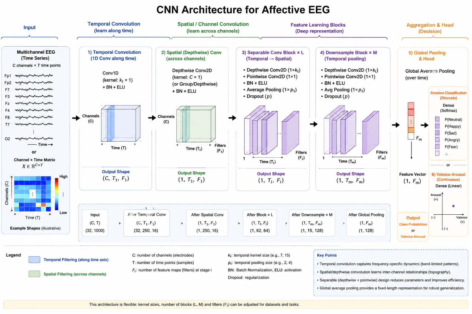
Figure 8.2: CNN architecture for affective EEG. Convolutional blocks learn local temporal and spatial EEG patterns before pooled feature maps are mapped to an affective prediction.
Theoretical Foundations
Convolution Operation
A 1D convolution applies a learnable filter (kernel) across the signal:
where is the input, is the filter weights, and is bias.
Variants of Convolution Operations
The basic convolution can be modified to control how information is mixed across channels, how much temporal context is observed, or how many parameters are used. Figure 8.3 summarizes representative variants. In EEG, the most useful distinction is between temporal filtering along the sample axis and channel mixing across electrodes or feature maps: an architecture should make this choice explicit rather than treating every axis of the input as an ordinary image dimension.
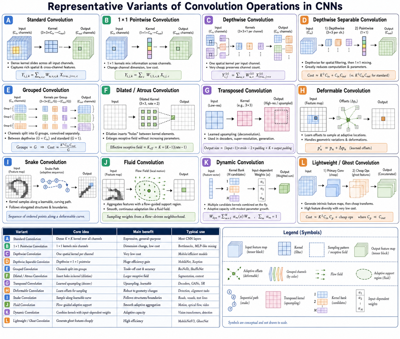
Figure 8.3: Representative variants of convolution operations. Each variant changes the receptive field, channel coupling, sampling locations, or computational cost of standard convolution. The lower table gives a compact comparison of the core idea and typical application of each operator.
Channel-mixing and efficient variants. A $1\times1$ pointwise convolution mixes feature channels without expanding the temporal or spatial receptive field; it is useful as a low-cost projection before or after a larger kernel. Depthwise convolution applies one filter to each channel independently, whereas depthwise separable convolution follows this with pointwise mixing. This separation is well suited to compact EEG models: temporal filters can first characterize each electrode or band, then a pointwise layer can learn cross-channel combinations. Grouped convolution offers an intermediate choice by restricting mixing to channel groups; it can encode electrode regions or frequency-band groups, but arbitrary groups should not be interpreted as neurophysiological networks without validation. Lightweight or ghost convolutions pursue a similar efficiency goal and are most relevant for wearable or latency-constrained deployment.
Receptive-field and resolution variants. Dilated (atrous) convolution spaces kernel elements apart, enlarging the effective receptive field without increasing the number of weights. It is useful when affect-related temporal context spans hundreds of milliseconds or seconds but the model must remain shallow. Transposed convolution performs learned upsampling, so it is primarily appropriate for decoders, reconstruction, segmentation, or generative EEG models—not ordinary trial-level classification. Both operators require careful checks for boundary effects and, for transposed convolution, uneven overlap artifacts.
Adaptive-sampling variants. Deformable convolution learns offsets from the regular sampling grid; snake and fluid convolutions similarly describe adaptive or path-guided sampling. Dynamic convolution combines multiple candidate kernels using input-dependent weights. These operations may help when informative EEG patterns vary in latency, topography, or morphology across trials, but they introduce additional flexibility and therefore a higher overfitting risk on the small datasets common in affective EEG. They should be evaluated against a standard or dilated convolution with matched capacity, subject-held-out splits, and computational cost reporting.
For most affective-EEG studies, start with standard temporal convolution plus a clearly defined spatial/channel-mixing layer. Depthwise-separable and dilated convolution are strong next ablations when efficiency or longer context is needed. More adaptive variants are research options rather than default choices: their added value should be demonstrated through controlled ablations and stability analyses.
Why Convolutions for EEG?
- Local connectivity: Neurons connect to nearby time points or adjacent channels
- Weight sharing: Same filter is applied across the signal (parameter efficiency)
- Hierarchical features: Lower layers learn simple patterns, higher layers combine them
- Translation invariance: Detects patterns regardless of position
Key Components
Convolutional Layer:
- Input: Multi-channel EEG signals
- Filters: Learnable feature detectors
- Output: Feature maps
Pooling Layer:
- Max pooling: Selects maximum value in region
- Average pooling: Computes average
- Reduces dimensionality and computational cost
- Provides translation invariance
Activation Functions:
- ReLU: Most common for intermediate layers
- Softmax: Classification outputs
- Tanh: Sometimes used for time-series
Adaptation to EEG-based Affective Computing
Signal Representation
EEG can be represented as a 2D input for CNNs:
Option 1: Channel × Time Matrix
Shape: (n_channels, n_samples)
Example: (14 channels, 2048 samples) = 14 × 2048 matrix
CNNs learn spatial patterns across channels and temporal patterns within time.
Option 2: Frequency × Time Spectrogram
Shape: (n_freq_bins, n_time_steps)
Example: (257 freq bins, 32 time frames) from STFT
CNNs learn frequency-temporal patterns similar to audio processing.
Option 3: 3D Input: Channel × Frequency × Time
Shape: (n_channels, n_freq_bins, n_time_steps)
Example: (14 channels, 30 freq bins, 64 time frames)
Most informative but computationally expensive.
Typical Pipeline
Raw EEG → Preprocessing → Segmentation → CNN → Emotion Label
           (Filtering)     (Windows)     (Automatic     (Valence/
                                         Feature        Arousal)
                                         Learning)
Suitable Input Features
Representation Choices
1. Raw Time-Series Signals
- Advantages:
- No information loss
- Let network learn optimal features
- Can capture high-frequency artifacts
- Disadvantages:
- Requires more data
- Noise-sensitive
- Longer training time
Example input:
# Shape: (batch_size, n_channels, n_samples)
# (32, 14, 2048)  # 32 samples, 14 channels, ~8 seconds at 256 Hz
2. Spectrogram Representation (Time-Frequency)
- Advantages:
- Emphasizes frequency content
- Robust to noise
- Mimics human auditory perception
- Good for emotional frequency bands
- Disadvantages:
- Information loss from time-frequency trade-off
- Requires STFT parameter tuning
Common parameters:
Window size: 256 samples
Hop length: 64 samples (75% overlap)
FFT size: 512
Output: 257 frequencies × ~30 time frames
3. Filtered Band-Specific Signals
Input channels:
- Delta band (0.5-4 Hz)      → 1 channel
- Theta band (4-8 Hz)        → 1 channel
- Alpha band (8-13 Hz)       → 1 channel
- Beta band (13-30 Hz)       → 1 channel
- Gamma band (30-100 Hz)     → 1 channel

Total: 5 × 14 channels = 70 channels per time sample
This preserves frequency information while reducing computational cost.
4. Differential Montage
Referential channels (14): Each referenced to average
Bipolar channels (13): Channel i - Channel i+1
Montage choice affects what spatial patterns CNNs can learn.
Preprocessing for CNNs
Unlike MLPs, preprocessing for CNNs emphasizes signal quality over feature engineering:
Minimal filtering: Preserve raw signal structure
- High-pass: 0.5-1 Hz (remove drift)
- Low-pass: 40-100 Hz (remove extreme noise)
- Avoid narrow bandpass if using raw signals
Artifact handling:
- Remove severely corrupted segments
- ICA-based component removal
- Or let network learn robustness
Normalization: Per-channel or per-segment
# Per-segment normalization (before passing to CNN) segment_norm = (segment - segment.mean()) / segment.std()Segmentation: Fixed-length windows
- Window size: 2-10 seconds
- Balance between temporal resolution and training speed
- Overlap: 50% common for more training samples
Network Architecture for EEG
Shallow CNN (Low Data Regime)
Input: (14 channels, 2048 time samples)
   ↓
Conv1D(32 filters, kernel=64, stride=4) → ReLU
   ↓
MaxPool1D(pool=4)
   ↓
Flatten
   ↓
Dense(128) → ReLU → Dropout(0.5)
   ↓
Output (emotion class)
Use when: Limited data (<1000 samples) or computational constraints.
Medium CNN (Balanced)
Input: (14 channels, 2048 time samples)
   ↓
Conv1D(64 filters, kernel=32) → BatchNorm → ReLU → MaxPool(4)
   ↓
Conv1D(128 filters, kernel=16) → BatchNorm → ReLU → MaxPool(4)
   ↓
Conv1D(256 filters, kernel=8) → BatchNorm → ReLU → MaxPool(2)
   ↓
GlobalAveragePooling1D()
   ↓
Dense(128) → ReLU → Dropout(0.5)
   ↓
Output (emotion class)
Use when: Moderate data (1000-5000 samples) and computational resources.
Deep CNN (High Data Regime)
Input: (14 channels, 2048 time samples)
   ↓
[Residual Block 1]
  Conv1D(32) → BatchNorm → ReLU
  Conv1D(32) → BatchNorm → ReLU
  + Residual connection
   ↓
[Residual Block 2]
  Conv1D(64) → BatchNorm → ReLU
  Conv1D(64) → BatchNorm → ReLU
  + Residual connection, Stride=2
   ↓
[Residual Block 3]
  Conv1D(128) → BatchNorm → ReLU
  Conv1D(128) → BatchNorm → ReLU
  + Residual connection, Stride=2
   ↓
GlobalAveragePooling1D()
   ↓
Dense(128) → ReLU → Dropout(0.5)
   ↓
Output (emotion class)
Use when: Large data (5000+ samples) with sufficient computational resources.
Spatial-Temporal CNN
Learns both channel relationships (spatial) and temporal patterns:
Input: (14 channels, 2048 time samples)
   ↓
# Spatial: Learn across channels
Conv1D(1, kernel=1) for each channel pair
   ↓
# Temporal: Learn across time
Conv1D(64, kernel=32)
   ↓
Conv1D(128, kernel=16)
   ↓
GlobalAveragePooling1D()
   ↓
Dense(128) → ReLU → Dropout(0.5)
   ↓
Output (emotion class)
Spectrogram-Based CNN (ResNet-style)
For 2D spectrograms (frequency × time):
Input: (14 channels, 257 frequencies, 64 time frames)
       Treat as grayscale image
   ↓
Conv2D(64, kernel=(3,3)) → ReLU → MaxPool(2,2)
   ↓
Conv2D(128, kernel=(3,3)) → ReLU → MaxPool(2,2)
   ↓
Conv2D(256, kernel=(3,3)) → ReLU → GlobalAveragePooling2D()
   ↓
Dense(256) → ReLU → Dropout(0.5)
   ↓
Output (emotion class)
Implementation Considerations
Filter Sizes and Receptive Field
Receptive field: The portion of input that influences one output neuron.
For EEG sampled at 250 Hz:
- To capture 1-second interactions: kernel ≥ 250
- To capture 2-second interactions: kernel ≥ 500
- Typical: kernels 64-256 for medium windows
Channel Dimension Handling
Option 1: Channels as input dimension (standard 1D CNN)
# Shape: (batch, time, channels)
Conv1D(filters, kernel_size)
Option 2: Channels as separate layers
# Apply Conv1D to each channel independently, then combine
# This reduces inter-channel information but speeds up training
Option 3: Spatial convolution across channels
# Treat (channels, time) as (height, width) for Conv2D
# Learns relationships between channels
Conv2D(filters, kernel=(3,1))  # kernel=(channels, time)
Preventing Overfitting
- Dropout: 0.3–0.5 after pooling or dense layers
- Batch Normalization: Stabilizes training, reduces overfitting
- Data augmentation:
- Time shifting
- Frequency band filtering variations
- Gaussian noise addition
- Temporal smoothing variations
- Early stopping: Monitor validation loss
Output Layer Design
For multiclass emotion classification:
Dense(num_emotions, activation='softmax')
loss = 'categorical_crossentropy'
For multi-label (multiple emotions simultaneously):
Dense(num_emotions, activation='sigmoid')
loss = 'binary_crossentropy'
For regression (valence/arousal continuous):
Dense(2, activation='linear')  # Output: [valence, arousal]
loss = 'mse'
Example Application: Valence-Arousal Prediction
Task
Predict continuous valence and arousal values from EEG.
Architecture
from tensorflow.keras import Sequential, layers

model = Sequential([
    # Input: (14 channels, 2048 samples)
    layers.Input(shape=(2048, 14)),

    # Conv blocks
    layers.Conv1D(64, kernel_size=32, padding='same'),
    layers.BatchNormalization(),
    layers.Activation('relu'),
    layers.MaxPooling1D(pool_size=4),
    layers.Dropout(0.3),

    layers.Conv1D(128, kernel_size=16, padding='same'),
    layers.BatchNormalization(),
    layers.Activation('relu'),
    layers.MaxPooling1D(pool_size=4),
    layers.Dropout(0.3),

    # Dense layers
    layers.GlobalAveragePooling1D(),
    layers.Dense(128, activation='relu'),
    layers.Dropout(0.5),
    layers.Dense(64, activation='relu'),
    layers.Dropout(0.3),

    # Output
    layers.Dense(2, activation='linear')  # [valence, arousal]
])

model.compile(
    optimizer='adam',
    loss='mse',
    metrics=['mae']
)
Preprocessing
# 1. Load raw EEG
signal = load_eeg_data()  # (14, 250000)

# 2. Filter
signal = bandpass_filter(signal, 0.5, 40)

# 3. Segment (8-second windows, 50% overlap)
segments = segment_signal(signal, window=2048, overlap=0.5)

# 4. Normalize per-segment
segments = np.array([
    (seg - seg.mean(axis=1, keepdims=True)) /
    (seg.std(axis=1, keepdims=True) + 1e-6)
    for seg in segments
])

# 5. Train
model.fit(segments, valence_arousal_labels,
          epochs=100, batch_size=32, validation_split=0.2)
Advantages and Disadvantages
| Aspect | CNNs | MLPs | RNNs |
|---|---|---|---|
| Automatic feature learning | ✓ Yes | ✗ No | ✓ Yes |
| Temporal modeling | Local (implicit) | Global (if available) | Global (explicit) |
| Spatial relationships | ✓ Channels | ✗ No | ✗ No |
| Computational cost | Medium | Low | High |
| Data requirements | Medium-high | Low-medium | High |
| Interpretability | Medium (filters visualizable) | High | Low |
| Real-time inference | Fast | Very Fast | Medium |
Comparison with Other EEG Analysis Methods
| Method | Feature Engineering | Performance | Inference Speed |
|---|---|---|---|
| Traditional ML (SVM, LDA) | High manual work | Good baseline | Very fast |
| MLP with hand-crafted features | Medium work | Good | Fast |
| CNN from raw signals | Minimal | Often superior | Medium-fast |
| LSTM from raw signals | Minimal | Often superior | Slow |
| Hybrid architectures | Minimal | State-of-the-art | Medium |
Best Practices
- Start with preprocessing: Even "raw" signals need filtering
- Experiment with input representation: Spectrogram vs. raw signals
- Use data augmentation: Especially with limited EEG data
- Validate generalization: Use LOSO (leave-one-subject-out) validation
- Visualize learned filters: Understand what the network learns
- Monitor for overfitting: Track train/validation loss divergence
Summary
Convolutional Neural Networks offer a powerful middle ground for EEG-based affective computing:
- Automatic feature extraction from raw or preprocessed signals
- Capture spatial patterns across channels
- Capture temporal patterns within windows
- Better data efficiency than RNNs
- Faster than RNNs for inference
CNNs work best when you have:
- Raw EEG signals or spectrograms
- Moderate to large datasets (500+ samples)
- Clear local patterns (within-channel or cross-channel)
- Reasonable computational resources
For modeling explicit temporal dependencies across the entire session or for variable-length sequences, RNNs become more suitable (see next section).
Next: Recurrent Neural Networks and LSTMs
References
- LeCun, Y., Bottou, L., Bengio, Y., and Haffner, P. (1998). Gradient-based learning applied to document recognition. Proceedings of the IEEE, 86(11), 2278–2324.
- Schirrmeister, R. T., Springenberg, J. T., Fiederer, L. D. J., et al. (2017). Deep learning with convolutional neural networks for EEG decoding and visualization. Human Brain Mapping, 38(11), 5391–5420.
- Lawhern, V. J., Solon, A. J., Waytowich, N. R., Gordon, S. M., Hung, C. P., and Lance, B. J. (2018). EEGNet: A compact convolutional neural network for EEG-based brain–computer interfaces. Journal of Neural Engineering, 15(5), 056013.
- Dose, H., Møller, J. S., Iversen, H. K., and Puthusserypady, S. (2018). An end-to-end deep learning approach to MI-EEG signal classification for BCIs. Expert Systems with Applications, 114, 532–542.
- Ding, Y., Robinson, N., Zhang, S., Zeng, Q., and Guan, C. (2022). TSception: Capturing temporal dynamics and spatial asymmetry from EEG for emotion recognition. IEEE Transactions on Affective Computing, 13(4), 2232–2245.