Structured Geometry of Emotion Spaces
Emotion labels are often represented as points in a flat Euclidean space: valence and arousal form a plane, and discrete emotions are treated as unrelated class identifiers. These choices are convenient, but they may discard meaningful structure. Affective states can have hierarchical, asymmetric, clustered, and context-dependent relationships; transitions between states may follow curved paths rather than straight lines; and discrete categories can be related by overlap, opposition, intensity, or transition likelihood.
Structured geometry offers a way to encode these relationships directly in the representation and prediction space. This section concerns the geometry of emotion states and labels, not the geometry of EEG sensor connectivity. The two can be combined, but they answer different questions.
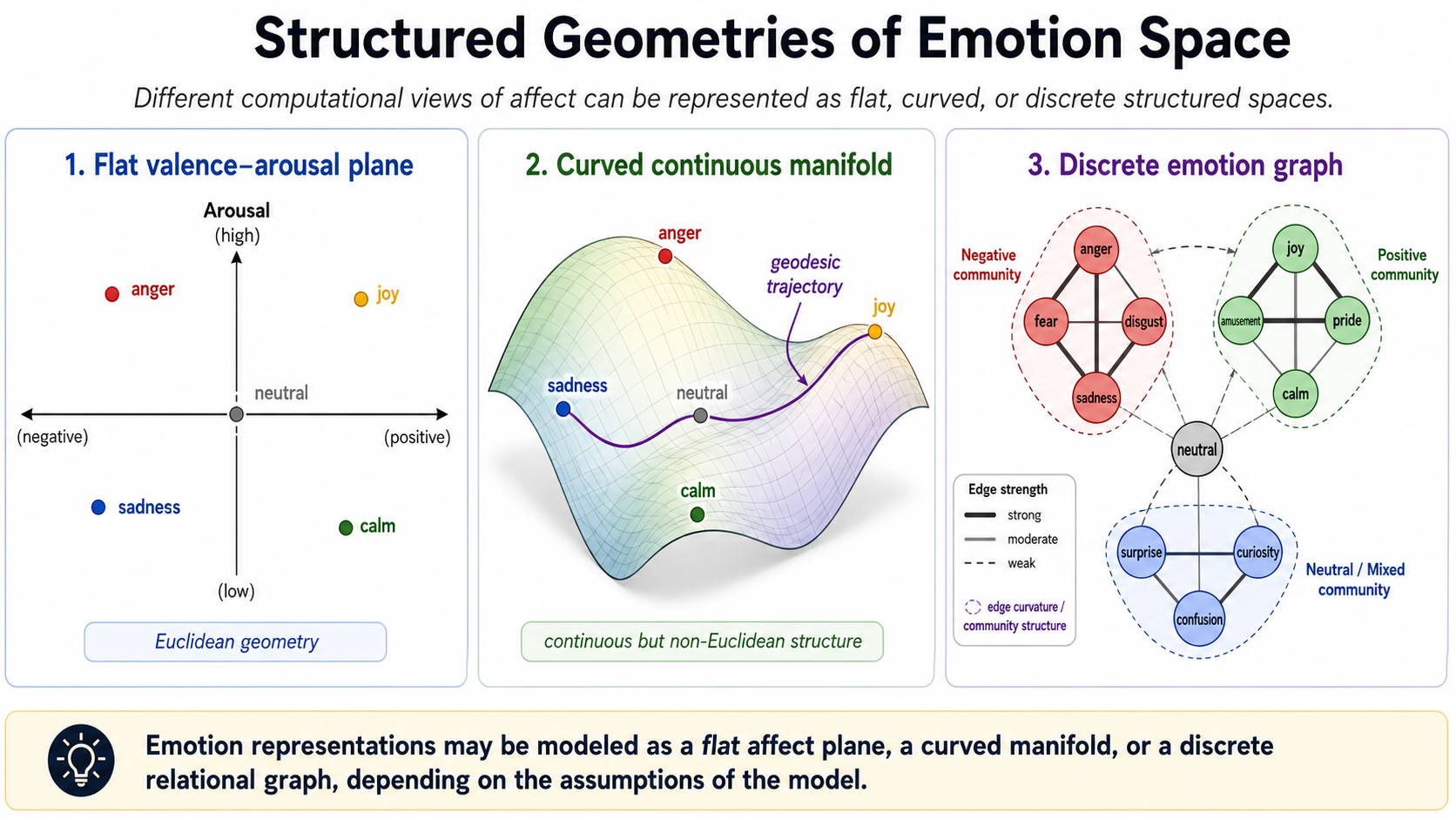
Figure 1. Structured geometry of emotion spaces. Flat coordinates, curved manifolds, and discrete graphs each encode different assumptions about how affective states relate to one another.
Why Flat Emotion Spaces Can Be Limiting
The familiar valence-arousal model provides a valuable low-dimensional coordinate system, but its Euclidean distance assumes that every direction and location has the same geometry. In a flat space, the shortest path between states is a straight line, local neighborhoods have equal capacity everywhere, and all pairs of coordinates have the same metric interpretation.
These assumptions may be too simple for some affective tasks. For example:
- high-arousal negative states may be easier to confuse with one another than with low-arousal negative states;
- broad affective families may branch into more specific states, producing hierarchy rather than a uniform plane;
- transitions may follow habitual or context-constrained routes rather than straight-line interpolation;
- and personal baselines may occupy different regions or use different local scales of the same space.
A curved representation is not automatically more psychologically valid. It is an inductive bias that must be compared with a Euclidean baseline and justified by improved prediction, calibration, interpretability, or generalization.
Continuous Affect on Non-Euclidean Manifolds
Let a continuous affective state be represented by a point on a manifold with metric . The metric determines local distance, angle, and the shortest path, or geodesic, between states. Curvature describes how this geometry differs from a flat Euclidean space.
| Geometry | Curvature | Useful structural bias | Potential affective interpretation |
|---|---|---|---|
| Euclidean | Uniform, flat coordinate space | Standard valence-arousal or valence-arousal-dominance regression | |
| Hyperbolic | Negative | Efficient representation of trees and expanding hierarchies | Broad affect families branching into more specific, context-dependent states |
| Spherical | Positive | Compact spaces with cyclic or globally bounded structure | Bounded, recurring affective configurations or directional state representations |
| Learned or variable curvature | Changes across the space | Different local regions can have different geometry | Dense, highly confusable regions and sparse, separable regions of emotion space |
Hyperbolic spaces are particularly useful when the structure is hierarchical. In a Poincare-ball representation, points near the center can encode general affective families, while points near the boundary represent increasingly specific states. Distance grows rapidly near the boundary, which can separate fine-grained leaves without requiring a high-dimensional Euclidean embedding.
Spherical spaces can be useful when affect is modeled as a bounded direction or when cyclic structure is more appropriate than unbounded coordinates. They should not be assumed merely because the traditional circumplex is drawn as a circle: a circular plot is a visualization choice, whereas a spherical manifold is a specific metric assumption.
The term parabolic emotion space needs care. A paraboloid is a curved surface with location-dependent positive curvature, but "parabolic" is not usually used as a standard constant-curvature alternative alongside Euclidean, hyperbolic, and spherical geometry. If affective data suggest different curvature in different regions, a learned Riemannian metric, product manifold, or variable-curvature latent space is the more precise formulation.
Geodesic Dynamics for Continuous Emotion
A trajectory in a curved latent space should be regularized by geodesic rather than ordinary Euclidean distance. For consecutive states and , a geometry-aware smoothness loss can be written as
where is the manifold distance. This lets smoothness respect the chosen geometry. A trajectory can move a small geodesic distance even when its coordinates change nonlinearly in a chart.
Models can combine an EEG encoder with a manifold-valued state head, Riemannian recurrent dynamics, or a latent state-space model. Predictions can be mapped to a Euclidean reporting scale when a dataset requires valence-arousal scores, while the internal representation retains curved structure.
Example scenario: A model learns from continuous ratings and EEG over several emotion-induction sessions. A Euclidean head predicts valence and arousal directly; a hyperbolic head represents a hierarchy from broad positive/negative states to more specific excited, calm, tense, and sad states. Both are evaluated with the same held-out subjects. The curved model is useful only if it improves held-out likelihood, trajectory calibration, or label-neighborhood consistency, not merely because its visualization appears more organized.
Discrete Emotion as a Graph
Discrete categories need not be independent output indices. They can be represented by a graph in which nodes are emotion concepts and weighted edges encode a declared relation. Possible relations include psychological similarity, valence-arousal proximity, transition probability, shared appraisal patterns, semantic association, or empirical confusion.
| Edge meaning | Example relation | Modeling use |
|---|---|---|
| Similarity | Fear and anxiety share negative valence and arousal | Graph-aware label smoothing or metric loss |
| Hierarchy | Negative affect contains fear, anger, sadness, and disgust | Hierarchical classification and coarse-to-fine prediction |
| Transition | Calm may transition to boredom more often than to panic in one task | Structured temporal decoding |
| Opposition | Joy and sadness have contrasting affective profiles | Margin constraints and error analysis |
| Context dependence | Frustration and engagement can co-occur during learning | Conditional or multiplex graphs rather than one fixed taxonomy |
The graph should be versioned and justified. A graph derived from a psychological theory is different from one learned from label co-occurrence or model confusion. Graph structure can guide a model, but it must not be mistaken for universal truth across cultures, tasks, or individuals.
Graph Curvature for Discrete Emotion Structure
Graph curvature quantifies the local geometry of a discrete emotion graph. Ollivier-Ricci curvature compares the neighborhoods of connected nodes through optimal transport, while Forman-Ricci curvature gives a simpler combinatorial measure. For an edge , Ollivier-Ricci curvature can be written as
where and are local neighborhood distributions, is Wasserstein distance, and is graph distance.
Positive curvature often indicates tightly connected local communities; negative curvature can indicate bridges, branching, or bottlenecks; near-zero curvature is more locally flat. In an emotion graph, these quantities can help identify:
- tightly related emotion families that may share representations;
- bridge states linking otherwise separate regions of the taxonomy;
- labels likely to be confused because they occupy the same local community;
- and bottleneck concepts whose removal disconnects high-level affect families.
Graph curvature here describes the structure of the label graph, not a neural mechanism. It should not be interpreted as evidence that the brain itself has the same geometry.
Geometry-Aware Model and Loss Design
Structured emotion spaces can enter a model at several levels:
- Geometry-aware output heads: Map EEG embeddings to manifold-valued continuous states or graph-structured discrete distributions.
- Distance-aware losses: Penalize errors by geodesic distance or graph distance, so confusing sadness with grief is treated differently from confusing sadness with joy when the task justifies that relation.
- Hierarchical decoding: Predict a coarse affect family before a fine-grained category, with consistency constraints across levels.
- Graph neural label encoders: Learn category embeddings through the emotion graph and use them in a classifier, zero-shot model, or prototype-based decoder.
- Curvature-aware regularization: Preserve local graph communities while allowing negative-curvature bridge edges to communicate information across emotion families.
- Temporal structured decoding: Penalize implausible graph jumps and favor transitions supported by context and uncertainty.
A graph neural network over emotion labels is distinct from a GNN over EEG channels. The first models relations among target states; the second models relations among sensors or sources. A joint model may use both, but its two graphs should be kept conceptually and empirically separate.
Evaluation and Interpretability
A non-Euclidean or graph-based emotion model should be evaluated against an equal-capacity Euclidean or independent-label baseline. Useful tests include:
| Claim | Evaluation |
|---|---|
| Better continuous representation | Held-out geodesic error, likelihood, calibration, and trajectory quality |
| Meaningful discrete structure | Agreement with independently specified taxonomy or transition data |
| Improved fine-grained recognition | Per-class recall, graph-distance-weighted error, and confusion reduction |
| Better generalization | Cross-subject, cross-session, or cross-context comparison with fixed geometry |
| Stable geometry | Curvature and neighborhood stability across resampling, subjects, and datasets |
| Faithful interpretation | Perturb label-graph edges or geometry and test whether predicted changes occur |
Do not select a geometry solely because it improves training loss or creates an attractive two-dimensional plot. Curvature, graph edges, and manifold coordinates are model assumptions. They become interpretable only when they are stable, externally grounded, and useful on data not used to construct them.
Practical Recommendations
- Start with a strong Euclidean baseline and a clearly defined psychological theory or data-derived graph.
- Match geometry to the hypothesized structure: use hyperbolic space for hierarchy, spherical space for bounded directional structure, and learned curvature only when data support the additional flexibility.
- Keep continuous geometry, discrete label graphs, and EEG connectivity graphs as separate objects with separate claims.
- Fit graph structure, curvature parameters, and loss weights using training data; evaluate all structural claims on held-out subjects, sessions, or datasets.
- Report edge definitions, curvature method, manifold parameterization, optimization details, and sensitivity to graph or geometry choices.
- Treat personal and cultural variation as a reason to test adaptable or multi-graph models, not as noise to erase.
Structured geometry will not settle the correct taxonomy of emotion. Its contribution is more modest and more useful: it gives models a language for representing nonuniform distances, hierarchy, transitions, and uncertainty that flat label spaces often hide.
References
- Russell, J. A. (1980). A circumplex model of affect. Journal of Personality and Social Psychology, 39(6), 1161-1178.
- Nickel, M., and Kiela, D. (2017). Poincare embeddings for learning hierarchical representations. Advances in Neural Information Processing Systems, 30.
- Ganea, O.-E., Becigneul, G., and Hofmann, T. (2018). Hyperbolic neural networks. Advances in Neural Information Processing Systems, 31.
- Bronstein, M. M., Bruna, J., LeCun, Y., Szlam, A., and Vandergheynst, P. (2017). Geometric deep learning: Going beyond Euclidean data. IEEE Signal Processing Magazine, 34(4), 18-42.
- Ollivier, Y. (2009). Ricci curvature of Markov chains on metric spaces. Journal of Functional Analysis, 256(3), 810-864.
- Forman, R. (2003). Bochner's method for cell complexes and combinatorial Ricci curvature. Discrete and Computational Geometry, 29, 323-374.