Graph Neural Networks (GNNs) for EEG-based Affective Computing
Overview
Graph Neural Networks represent a paradigm shift in modeling EEG data by explicitly leveraging the spatial structure of brain networks. Unlike CNNs that treat channels as a sequence or Transformers that ignore spatial relationships, GNNs model EEG channels as nodes in a graph with connections based on functional or anatomical brain connectivity. This section explores how GNNs can capture the graph structure of brain networks for improved emotion recognition.
Graph Neural Network Architecture
A graph neural network represents data as a set of nodes, their features, and the edges that specify which nodes can exchange information. Instead of applying the same local filter over a regular grid, as a CNN does, a GNN performs message passing: every node collects and aggregates messages from its neighbors, combines them with its own representation, and passes the result through a learnable transformation. Repeating this process lets each node incorporate information from progressively larger parts of the graph.
The main design decisions are therefore the graph structure and the aggregation rule. Edges may be fixed from prior knowledge, computed from similarity, or learned from data; they may also carry weights that quantify connection strength. A graph-convolution layer commonly averages or normalizes neighbor features, whereas graph attention learns how much weight to give each neighbor. After several message-passing layers, a pooling or readout operation combines node representations into a graph-level embedding for classification, regression, or other downstream tasks.
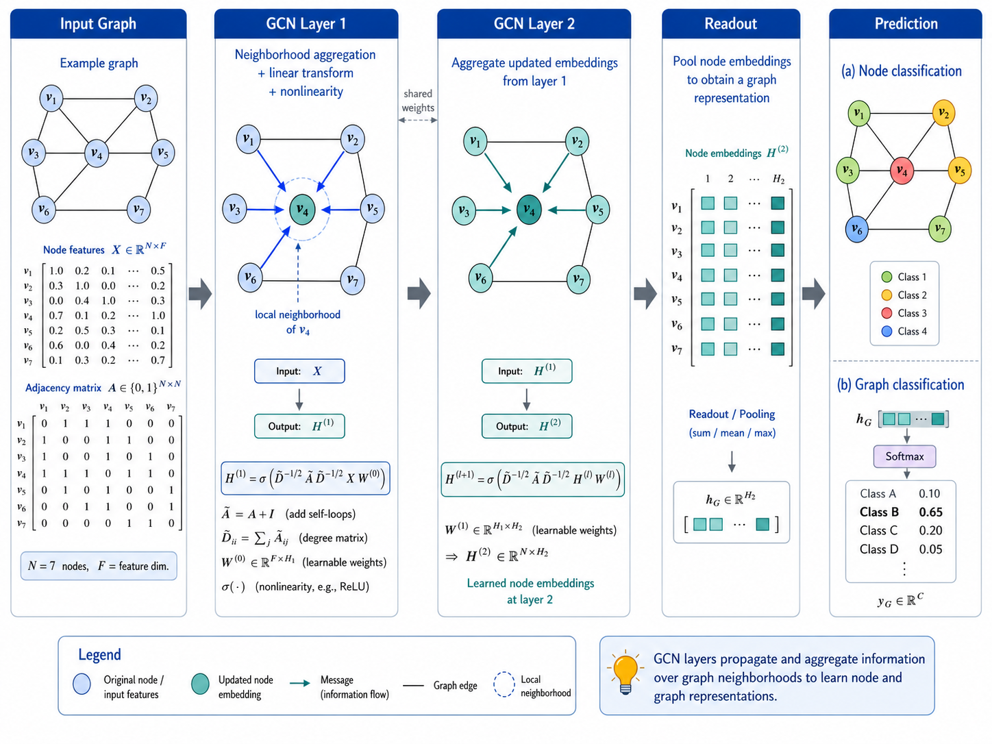
Figure 8.6: Graph neural network architecture. Node features are exchanged along graph edges through message passing, then pooled into a graph representation for a downstream prediction task.
Theoretical Foundations
Graph Representation
A graph consists of:
- Vertices (Nodes): - EEG channels/electrodes
- Edges: - Connections between channels based on brain connectivity
- Node features: - EEG signals or spectral features
- Adjacency matrix: - Connection weights between channels
For EEG with 14 channels:
n = 14 (nodes = electrodes)
d = temporal resolution (features per node)
A = 14 × 14 adjacency matrix (brain connectivity)
Graph Convolution
Graph convolution generalizes standard convolution to irregular graph structures:
Spectral approach (using graph Laplacian):
where:
- = node features at layer
- = adjacency matrix
- = degree matrix ()
- = learnable weights
- = activation function
Spatial approach (message passing):
where:
- = neighbors of node
- = feature vector of node at layer
- Message is aggregated from all neighbors
GNN Architectures
GNN variants differ primarily in how they decide which neighbor information to aggregate and how much expressiveness they retain (Figure 8.7). GCN uses normalized fixed-weight aggregation as an efficient baseline; GAT learns attention weights for each connection; GraphSAGE defines an inductive sample-and-aggregate scheme; and GIN uses an MLP-based update designed to distinguish a wider range of graph structures. For EEG, the choice reflects a trade-off between stable use of a prior connectivity graph, adaptive task-relevant connectivity, and the risk of overfitting a limited number of subjects.
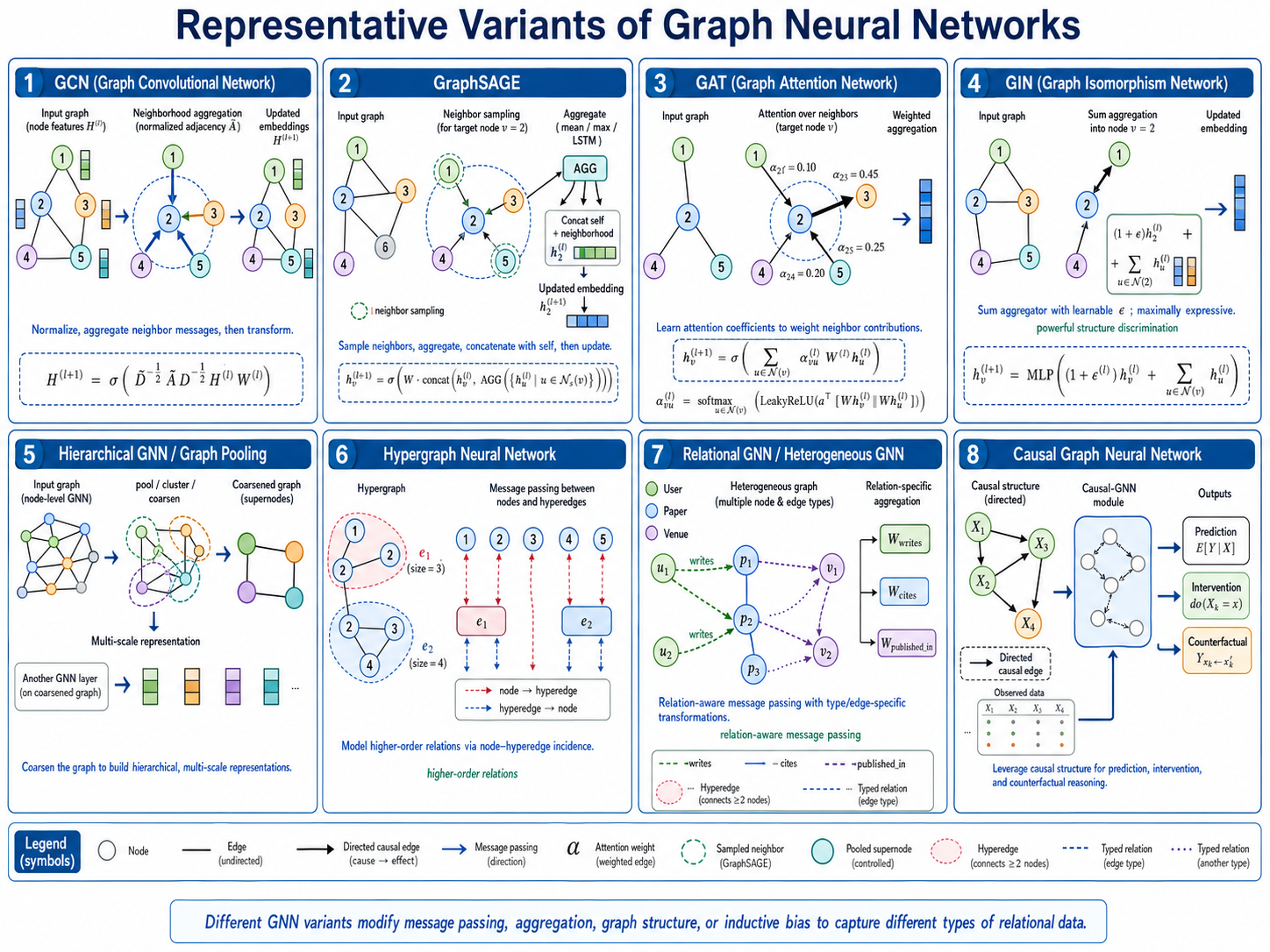
Figure 8.7: Graph neural network variants. GCN aggregates normalized neighbor features, GAT learns attention-weighted aggregation, GraphSAGE samples and aggregates local neighborhoods, and GIN uses a highly expressive MLP-based aggregation rule.
Graph Convolutional Network (GCN)
Simplest GNN, using spectral convolutions:
where is normalized adjacency matrix.
Advantages:
- Computationally efficient
- Well-understood and stable
- Good baseline for brain networks
Disadvantages:
- May oversmooth for deep networks
- Limited expressiveness with fixed weights
Graph Attention Networks (GAT)
Uses attention mechanisms to weight neighbor contributions:
Attention weights:
Advantages:
- Learns which connections are important
- Multi-head attention for stability
- Interpretable attention weights
GraphSAGE (Sample and Aggregate)
Learns to aggregate neighbor information:
Aggregation functions:
- Mean:
- LSTM:
- Pooling:
Graph Isomorphism Network (GIN)
More expressive than GCN:
where is a learnable parameter.
Adaptation to EEG-based Affective Computing
Why GNNs for EEG?
Advantages:
- Explicit brain structure: Leverages functional or anatomical connectivity
- Irregular topology: Handles electrode positions without spatial regularity
- Learnable connections: Can discover task-relevant connections
- Multi-scale analysis: Hierarchical networks capture nested structure
- Interpretability: Attention weights show channel importance
Challenges:
- Graph construction: How to define edges? (correlation, coherence, anatomical?)
- Dynamic graphs: Brain connectivity changes over time
- Limited labeled data: GNNs often need large graphs; EEG has only ~14-64 channels
- Computational overhead: Graph operations add complexity
- Hyperparameter sensitivity: GNNs can be difficult to tune
Graph Construction from EEG
Option 1: Anatomical Connectivity
Based on known brain structure:
Create fixed edges based on electrode proximity:
- Fp1, Fp2 (frontal poles) → connected to F3, F4 (frontal)
- F3, F4 → connected to C3, C4 (central)
- C3, C4 → connected to P3, P4 (parietal)
- P3, P4 → connected to O1, O2 (occipital)
- etc. (Standard 10-20 electrode system)
Pros: Fixed, interpretable, domain-guided Cons: Ignores task-specific connectivity
Option 2: Functional Connectivity
Based on signal relationships during task:
Pearson Correlation:
Simple but can be noisy.
Coherence:
Frequency-specific relationship (0 ≤ coherence ≤ 1).
Wavelet Coherence:
Time-frequency dependent relationships.
Mutual Information:
Captures non-linear relationships.
Phase Synchrony:
Phase lag index (robust to volume conduction).
Option 3: Hybrid Connectivity
Combine anatomical and functional:
where and are weights.
Option 4: Learnable Connectivity
Let the network learn edge weights:
Input: raw or spectral EEG
↓
Compute pairwise similarity between channels
↓
Learnable edge weights (parameterized)
↓
Input to GNN
Advantage: Task-specific connections Disadvantage: May overfit, harder to interpret
Threshold for Edge Creation
For sparse graphs (especially with ~14 channels):
# Keep top-k connections per node
A_sparse = keep_topk(A, k=5)

# Or threshold-based
A_sparse[A < threshold] = 0

# Or statistical significance
A_sparse[p_value > 0.05] = 0
This reduces noise and computational cost.
Suitable Input Features
Node Feature Options
Option 1: Raw Time-Series per Channel
# Each node (channel) has temporal features
X shape: (n_channels, n_samples)
# Example: (14, 2048)

# GNN processes:
# - Node i = Channel i (1000+ samples at 256 Hz)
# - Edges = Brain connectivity
# - Output = Emotion prediction

# Challenge: Long sequences, GNN processes all time steps
Option 2: Spectral Features per Channel
# Pre-extract frequency features for each channel
X shape: (n_channels, n_freq_bands)
# Example: (14, 5)
# 5 bands: Delta, Theta, Alpha, Beta, Gamma

# Much more efficient than raw signals
# Embeds frequency information in node features
Option 3: Spectral-Temporal Features
# Spectrogram per channel
X shape: (n_channels, n_time_frames, n_freq_bins)
# Example: (14, 32, 30)
# 32 time frames, 30 frequency bins per channel

# Requires 3D GNN or careful reshaping
# Captures time-frequency dynamics
Option 4: Statistical Features
# Hand-crafted features per channel
X shape: (n_channels, n_features)
# Example: (14, 20)
# Features: mean, variance, skewness, kurtosis, entropy, etc.

# Simplest and fastest
# Loses temporal information
Network Architecture for EEG
Simple GNN (Single Layer)
Input: (14 channels) with EEG signals/features
        (14 × 14) adjacency matrix
   ↓
GCN Layer (64 units)
   ↓
Global Average Pooling
   ↓
Dense(32) → ReLU
   ↓
Output (emotion class)
Use when: Limited data or computational resources.
Multi-Layer GNN
Input: EEG features (14, n_features)
       Adjacency matrix (14, 14)
   ↓
[GCN Block 1]
  GCN(64 units)
  BatchNorm
  ReLU
   ↓
[GCN Block 2]
  GCN(128 units)
  BatchNorm
  ReLU
   ↓
[GCN Block 3]
  GCN(64 units)
  BatchNorm
  ReLU
   ↓
Global Average Pooling
   ↓
Dense(128) → ReLU → Dropout(0.3)
   ↓
Dense(3, softmax) [emotion classes]
Graph Attention Network (GAT)
Input: EEG features (14, n_features)
       Adjacency matrix (14, 14)
   ↓
[Attention Layer 1]
  Multi-head attention (8 heads)
  Learn which channels matter
   ↓
[Attention Layer 2]
  Multi-head attention (8 heads)
   ↓
Global Average Pooling
   ↓
Dense(32) → ReLU
   ↓
Output
Advantage: See which channel interactions are important via attention weights.
Temporal GNN (Spatio-Temporal)
For dynamic graphs (connectivity changes over time):
Input: EEG signals (n_timesteps, n_channels)
   ↓
[For each time step]
  - Compute functional connectivity (adjacency matrix)
  - Apply GNN
  - Produces node embeddings at each time step
   ↓
LSTM on node embeddings across time
   ↓
Global Average Pooling
   ↓
Emotion prediction
Graph Pooling Layers
Hierarchical graph structure:
Input: Full graph (14 nodes)
   ↓
GNN Layer
   ↓
Graph Pooling: Reduce to 8 nodes
   ↓
GNN Layer
   ↓
Graph Pooling: Reduce to 4 nodes
   ↓
GNN Layer
   ↓
Global Pooling (1 representation)
   ↓
Dense layers
   ↓
Output
Pooling strategies:
- Top-k: Keep highest activation nodes
- Attention-based: Weight importance of nodes
- Clustering: Group similar nodes
Implementation Considerations
Graph Construction Algorithm
import numpy as np
from scipy.stats import pearsonr

def construct_adjacency_matrix(eeg_signal, method='correlation', threshold=0.5):
    """
    Construct adjacency matrix from EEG

    Args:
        eeg_signal: (n_channels, n_samples)
        method: 'correlation', 'coherence', 'phase_sync'
        threshold: connectivity threshold
    """
    n_channels = eeg_signal.shape[0]
    A = np.zeros((n_channels, n_channels))

    if method == 'correlation':
        for i in range(n_channels):
            for j in range(i+1, n_channels):
                corr, _ = pearsonr(eeg_signal[i], eeg_signal[j])
                A[i,j] = A[j,i] = max(0, corr)  # Keep positive correlations

    # Apply threshold
    A[A < threshold] = 0

    # Normalize (optional)
    A = A / (A.max() + 1e-6)

    return A
Handling Variable Graph Sizes
EEG typically has 14-64 channels, but graphs must be fixed size for neural networks:
Solution 1: Standardize electrode placement
# Use standard 10-20 system
# Always 14 or 19 channels in consistent positions
Solution 2: Interpolation to common grid
# Interpolate from actual electrode positions to fixed positions
# Ensures consistent graph structure
Solution 3: Padding
# Pad smaller graphs with dummy nodes (no connections)
Normalization of Adjacency Matrix
Different normalization strategies affect learning:
Symmetric normalization (standard):
Row normalization:
Adding self-loops:
Helps with gradient flow and stabilizes training.
Initialization and Training
Xavier initialization for graph layers:
weight.data.normal_(0, np.sqrt(2.0 / (in_features + out_features)))
Learning rate: Typically lower than CNNs
- GCN: 0.0001-0.001
- GAT: 0.001-0.01
Optimizer: Adam often works well
optimizer = Adam(learning_rate=0.001)
Example Application: Emotion Classification with GAT
Task
Classify EEG into emotional states using brain network structure.
Architecture
import torch
import torch.nn as nn
import torch.nn.functional as F
from torch_geometric.nn import GATConv, global_mean_pool

class EEGEmotionGAT(nn.Module):
    def __init__(self, n_channels=14, n_features=30, n_emotions=3):
        super().__init__()

        # Graph Attention layers
        self.gat1 = GATConv(n_features, 64, heads=4, concat=True)
        self.gat2 = GATConv(256, 128, heads=4, concat=True)  # 64×4=256 input
        self.gat3 = GATConv(512, 64, heads=1)  # 128×4=512 input

        # Classification head
        self.fc1 = nn.Linear(64, 32)
        self.fc2 = nn.Linear(32, n_emotions)
        self.dropout = nn.Dropout(0.3)

    def forward(self, x, edge_index):
        """
        Args:
            x: node features (14, n_features)
            edge_index: edge connectivity (2, n_edges)
        """
        # GAT layers with ReLU and dropout
        x = F.relu(self.gat1(x, edge_index))
        x = self.dropout(x)

        x = F.relu(self.gat2(x, edge_index))
        x = self.dropout(x)

        x = self.gat3(x, edge_index)

        # Global pooling (average across nodes)
        x = x.mean(dim=0)  # (64,)

        # Classification
        x = F.relu(self.fc1(x))
        x = self.dropout(x)
        x = self.fc2(x)

        return x
Data Preparation
import numpy as np
from torch_geometric.data import Data
import torch

def prepare_eeg_graph_data(eeg_signal, emotion_label):
    """
    Convert EEG to graph format

    Args:
        eeg_signal: (14, 2048) - channels × time samples
        emotion_label: scalar emotion class
    """
    # 1. Extract spectral features per channel
    node_features = []
    for ch in range(eeg_signal.shape[0]):
        features = extract_spectral_features(eeg_signal[ch])  # (30,)
        node_features.append(features)

    node_features = np.array(node_features)  # (14, 30)

    # 2. Construct adjacency matrix (functional connectivity)
    A = construct_adjacency_matrix(eeg_signal, method='correlation', threshold=0.3)

    # 3. Convert to edge index format
    edge_index = []
    for i in range(14):
        for j in range(14):
            if A[i,j] > 0:
                edge_index.append([i, j])

    edge_index = np.array(edge_index).T  # (2, n_edges)

    # 4. Create PyG Data object
    data = Data(
        x=torch.FloatTensor(node_features),
        edge_index=torch.LongTensor(edge_index),
        y=torch.LongTensor([emotion_label])
    )

    return data

def extract_spectral_features(signal, fs=256, bands=None):
    """Extract power in frequency bands"""
    if bands is None:
        bands = {'delta': (0.5, 4), 'theta': (4, 8), 'alpha': (8, 13),
                 'beta': (13, 30), 'gamma': (30, 100)}

    from scipy import signal as scipy_signal

    freqs, psd = scipy_signal.welch(signal, fs=fs, nperseg=256)

    features = []
    for band_name, (f_low, f_high) in bands.items():
        mask = (freqs >= f_low) & (freqs < f_high)
        band_power = psd[mask].mean()
        features.append(band_power)

    # Add statistical features
    features.extend([signal.mean(), signal.std(), signal.var()])

    return np.array(features)

# Training loop
model = EEGEmotionGAT()
optimizer = torch.optim.Adam(model.parameters(), lr=0.001)
criterion = nn.CrossEntropyLoss()

for epoch in range(100):
    for batch in data_loader:
        optimizer.zero_grad()

        out = model(batch.x, batch.edge_index)
        loss = criterion(out, batch.y)

        loss.backward()
        optimizer.step()
Advantages and Disadvantages
| Aspect | GNN | CNN | LSTM | Transformer |
|---|---|---|---|---|
| Brain structure | Explicit | Implicit | Implicit | Implicit |
| Interpretability | High (attention) | Medium | Low | High |
| Small graphs | Good fit | OK | OK | Overkill |
| Scalability | Limited (14-64 nodes) | Excellent | Good | Excellent |
| Temporal modeling | Weak (static graphs) | Good (local) | Excellent | Excellent |
| Data requirements | Medium (500+) | Medium-High | High | Very High |
| Training speed | Fast | Fast | Slow | Medium |
| Flexibility | High (custom graphs) | Medium | Low | Low |
Comparison: When to Use GNNs
GNNs are better when:
- ✓ Brain network structure is important
- ✓ Interpretability via channel importance is critical
- ✓ Data is limited (fewer parameters than CNN/RNN)
- ✓ Electrode positions/layout matters
- ✓ Want to visualize learned connectivity patterns
Prefer alternatives when:
- ✗ Temporal dynamics are primary focus (→ LSTM)
- ✗ Parallel processing critical (→ Transformer)
- ✗ Very long sequences needed (→ CNN)
- ✗ Transfer learning desired (→ CNN/Transformer)
- ✗ Computational efficiency paramount (→ MLP)
Advanced GNN Concepts for EEG
Dynamic Graph Neural Networks
Brain connectivity changes over time:
Time t₁: Compute connectivity matrix A₁
Time t₂: Compute connectivity matrix A₂
  ...
Time tₙ: Compute connectivity matrix Aₙ
   ↓
Apply GNN to each time-varying graph
   ↓
Aggregate temporal dynamics (LSTM, attention)
   ↓
Emotion prediction
Heterogeneous Graphs
Different node types (EEG channels + other sensor data):
Nodes:
- Type 1: EEG channels (14)
- Type 2: ECG data (1)
- Type 3: GSR data (1)

Edges:
- EEG-to-EEG: Brain connectivity
- EEG-to-ECG: Physiological coupling
- ECG-to-GSR: Peripheral coupling

→ Heterogeneous GNN with type-aware layers
Graph Contrastive Learning
Self-supervised approach:
1. Create two augmented graphs from same data:
   - Augmentation 1: Drop 20% of edges
   - Augmentation 2: Perturb features slightly

2. GNN encodes both: z₁ = GNN(G₁), z₂ = GNN(G₂)

3. Maximize similarity: similarity(z₁, z₂)

4. Fine-tune on emotion labels with pre-trained encoder
Discrete Curvature for EEG Graph Analysis
What Is Discrete Curvature?
In Riemannian geometry, curvature measures how a space deviates from being flat. Discrete curvature extends this idea to graphs, quantifying how "curved" local neighbourhoods are. Two common formulations are:
Ollivier-Ricci Curvature (ORC) compares the Wasserstein distance between probability distributions on neighbouring nodes to the shortest-path distance between the nodes themselves:
where and are probability measures concentrated around nodes and , is the 1-Wasserstein distance, and is the graph distance.
Interpretation:
- : locally "spherical" — tightly connected community
- : locally "flat" — grid-like structure
- : locally "hyperbolic" — tree-like or bottleneck structure
Forman-Ricci Curvature (FRC) is a simpler combinatorial alternative:
where is the edge weight and the sum runs over edges adjacent to .
Why Curvature Matters for EEG GNNs
Discrete curvature provides several insights for EEG graph modelling:
1. Detecting Bottlenecks and Oversquashing
Negative-curvature edges act as information bottlenecks in message-passing GNNs — a phenomenon known as oversquashing, where information from many nodes is compressed through a narrow pathway. In EEG graphs, this can reveal:
- critical hub channels through which emotional information flows,
- edges where gradient signals may be attenuated during training,
- structural weaknesses in the graph that limit model expressiveness.
2. Curvature-Guided Graph Rewiring
Edges with strongly negative curvature can be augmented or rewired to improve information flow:
# Compute ORC on the EEG connectivity graph
curvatures = compute_ollivier_ricci_curvature(A, node_features)

# Identify bottleneck edges (κ < -0.5)
bottleneck_edges = np.where(curvatures < -0.5)

# Rewiring: add new edges near bottlenecks to alleviate oversquashing
A_rewired = add_edges_near_bottlenecks(A, bottleneck_edges)
This can improve GNN performance without increasing model capacity.
3. Community Detection
Positive curvature regions correspond to tightly connected communities — functionally coupled brain regions. In EEG affective computing, curvature-based community detection can:
- identify which electrode groups co-activate during specific emotional states,
- reveal hierarchical brain network organization,
- provide interpretable functional modules for emotion processing.
4. Curvature as an Edge Feature
Curvature values can be used as additional edge features in GNNs:
# Augment adjacency with curvature-based edge weights
curvature_features = compute_forman_curvature(A)
edge_attr = curvature_features[edge_index]  # Shape: (n_edges,)

# Use in GNN message passing
x = GATConv(x, edge_index, edge_attr=edge_attr)
EEG-Specific Considerations
- Curvature computations are relatively expensive for large graphs, but EEG graphs are small (14-64 nodes), making curvature analysis tractable.
- Curvature depends on the graph construction method — functional connectivity yields very different curvature patterns than anatomical connectivity.
- Temporal curvature dynamics: as brain connectivity changes during emotional processing, curvature patterns shift, potentially identifying when emotion-relevant network reconfigurations occur.
Practical Recommendations
- Use Forman-Ricci curvature as a fast first-pass analysis; switch to Ollivier-Ricci for deeper structural insight.
- Compute curvature per emotional condition to see how network geometry differs across states.
- Use curvature not only for analysis but also as a regularization signal — penalize the model when important emotional edges have high bottleneck curvature.
- Visualize curvature on a topographic head plot with edges coloured by to reveal brain network geometry.
Causal Graphs for EEG Connectivity
From Correlation to Causation
Most EEG connectivity graphs are built on symmetric, undirected measures — correlation, coherence, phase synchrony. These capture statistical association but cannot distinguish:
- whether channel A drives channel B or vice versa,
- whether a third channel C confounds the A-B relationship,
- whether the association reflects genuine neural interaction or volume conduction.
Causal graph approaches address these limitations by constructing directed graphs where edges represent directional influence.
Causal Discovery Methods for EEG
Granger Causality tests whether past values of one time series improve prediction of another:
Spectral Granger causality extends this to frequency domain, directly linking to EEG bands:
from mne_connectivity import spectral_connectivity_epochs

# Compute directed connectivity in alpha band
con = spectral_connectivity_epochs(
    epochs, method='gc', sfreq=256, fmin=8, fmax=13
)
# con shape: (n_channels, n_channels) — directed adjacency
Transfer Entropy is an information-theoretic alternative sensitive to nonlinear interactions:
This is useful for EEG because neural interactions are often nonlinear.
Directed Information generalizes mutual information to directed settings, capturing the full temporal causal structure.
Conditional Independence Testing (PC Algorithm) discovers causal structure by testing for conditional independence between channel pairs.
Causal Graph Neural Networks
Once a causal (directed) graph is constructed, GNNs can be adapted:
1. Directed Message Passing
Standard GNNs assume undirected edges. For causal graphs:
# Use separate weight matrices for incoming vs. outgoing edges
h_v = σ(
    W_self @ h_v +
    W_in  @ aggregate({h_u: u → v}) +   # Incoming causal influence
    W_out @ aggregate({h_w: v → w})      # Outgoing causal influence
)
2. Causal Attention
Attention weights can be constrained by causal structure:
# Only attend to nodes that causally influence the target
α_{vu} = 0 if u does not Granger-cause v
This produces sparser, more interpretable attention patterns.
3. Structural Causal Models (SCM) with GNNs
Embed EEG causal graphs in an SCM framework:
z (exogenous) → h (endogenous) → y (emotion)
       ↑               ↑
   Causal GNN     Causal constraints
The GNN learns representations that respect the causal structure, improving out-of-distribution generalization and robustness to interventions.
Why Causal Graphs Matter for EEG Affective Computing
1. Avoiding Spurious Associations
Correlation-based connectivity can be inflated by:
- volume conduction (same source picked up by multiple electrodes),
- common reference effects,
- shared noise sources.
Causal analysis helps separate genuine neural interaction from these confounds.
2. Interpretability
Directed edges have a clear interpretation: "channel F3 causally influences channel F4 in the alpha band during high-valence states." This is more neuroscientifically meaningful than "F3 and F4 are correlated."
3. Intervention Reasoning
Causal models support "what-if" reasoning:
- What would the EEG pattern look like if we perturbed frontal activity?
- Which channels are causal drivers of the emotional response vs. downstream effects?
4. Cross-Subject Generalization
Causal relationships may be more invariant across subjects than correlational ones because they capture mechanistic influence rather than statistical association.
Practical Integration with GNNs
| Step | Method |
|---|---|
| 1. Causal Discovery | Granger causality, transfer entropy, or PC algorithm on EEG time series |
| 2. Graph Construction | Build directed adjacency matrix with thresholding |
| 3. GNN Adaptation | Directed message passing or causal attention masking |
| 4. Training | Train GNN with causal constraints (e.g., regularization based on causal structure) |
| 5. Evaluation | Test on held-out subjects; evaluate robustness to interventions |
Caveats and Limitations
- Granger causality assumes linearity — nonlinear extensions exist but are more complex.
- Causal discovery from observational data alone has fundamental limits; interventional data (e.g., TMS-EEG) is rarely available.
- Temporal resolution matters: EEG at 256 Hz may miss very fast causal interactions.
- Causal graphs add complexity to the GNN pipeline; the benefit must be weighed against increased computational and methodological overhead.
Best Practices for EEG GNNs
- Start with anatomical connectivity: Baseline before learning
- Thresholds wisely: Too sparse = disconnected graph; too dense = noise
- Normalize adjacency matrix: Affects gradient flow
- Use attention: Interpretability and adaptive weighting
- Combine with temporal: GNN + LSTM for full dynamics
- Validate connectivity: Ensure discovered connections make neurophysiological sense
- Regularize: Prevent overfitting with small graphs
- Visualize learned patterns: Show which connections the model uses
- Analyse curvature: Use discrete curvature (Ollivier-Ricci, Forman) to detect bottlenecks, guide rewiring, and uncover community structure in brain networks
- Consider causal graphs: Where temporal resolution permits, replace undirected correlation-based edges with directed causal edges (Granger, transfer entropy) for stronger interpretability and intervention reasoning
Summary
Graph Neural Networks offer a principled way to incorporate brain network structure into EEG-based emotion recognition:
Key Strengths:
- Explicit modeling of spatial brain organization
- Natural fit for electrode networks
- Interpretable learned importance of channel relationships
- Parameter-efficient compared to CNNs/RNNs
- Good for understanding what the model learns
Practical Limitations:
- Fixed small graphs (14-64 channels)
- Less effective for pure temporal modeling
- Less established transfer learning compared to CNNs
- Sensitive to graph construction method
- May require domain expertise in connectivity
When to Use:
- Neuroscience focus with interpretability requirements
- Small datasets with structural importance
- Multi-modal integration of brain regions
- Need to understand learned connectivity patterns
Future Directions:
- Dynamic graphs capturing time-varying connectivity
- Discrete curvature analysis for bottleneck detection and graph rewiring
- Causal graph construction and directed GNNs for interpretable brain networks
- Multi-scale hierarchical GNNs
- Combination with domain-specific priors
- Better transfer learning for EEG
- Integration with clinical knowledge
GNNs represent the natural evolution of EEG analysis toward explicitly incorporating neurobiological structure—a key advantage for clinical and research applications where interpretability and domain alignment are paramount.
Related Reading: See Hybrid Architectures and Advanced Models for combinations of GNNs with other approaches. For emerging paradigms, see Trending Architectures.
References
- Bruna, J., Zaremba, W., Szlam, A., and LeCun, Y. (2014). Spectral networks and locally connected networks on graphs. In ICLR.
- Kipf, T. N., and Welling, M. (2017). Semi-supervised classification with graph convolutional networks. In ICLR.
- Veličković, P., Cucurull, G., Casanova, A., Romero, A., Liò, P., and Bengio, Y. (2018). Graph attention networks. In ICLR.
- Wu, Z., Pan, S., Chen, F., Long, G., Zhang, C., and Yu, P. S. (2021). A comprehensive survey on graph neural networks. IEEE Transactions on Neural Networks and Learning Systems, 32(1), 4–24.
- Song, T., Zheng, W., Song, P., and Cui, Z. (2018). EEG emotion recognition using dynamical graph convolutional neural networks. IEEE Transactions on Affective Computing, 11(3), 532–541.
- Zhong, P., Wang, D., and Miao, C. (2020). EEG-based emotion recognition using regularized graph neural networks. IEEE Transactions on Affective Computing, 13(3), 1290–1301.
- Ollivier, Y. (2009). Ricci curvature of Markov chains on metric spaces. Journal of Functional Analysis, 256(3), 810–864.