Streaming Architecture and Time Semantics
A real-time affective BCI is a timed pipeline. Samples leave sensors, acquire timestamps, cross a transport, wait in buffers, become windows, become features or embeddings, become predictions, become policy decisions, and finally become interface events that the user can perceive. Each stage has its own delay. Confusing those delays, or treating a device clock as identical to physiological time, is how an apparently online system becomes an offline analysis with a live display.
This section specifies the path from sensors to action and the several meanings of "time" along that path. Filter causality, window design, and chronological evaluation are defined in Chapter 6 and Chapter 9. Here the question is architectural: how the system is wired so those constraints can be kept.
From Sensors to Action
A complete path typically includes:
- Acquisition. Electrodes, amplifiers, and any auxiliary sensors (EOG, EMG, heart rate, motion, audio, eye tracking) convert physical processes into digital samples.
- Timestamping. Each sample or chunk is associated with a clock reading. That reading may originate on the device, on the acquisition computer, or on a receiver after network transport.
- Transport. Samples move over USB, Bluetooth, Wi-Fi, a local network, or an in-process queue. Transport can reorder, duplicate, delay, or drop data.
- Buffering. A ring buffer or timestamp-indexed store holds a finite history so that windows can be formed without blocking acquisition.
- Preprocessing. Referencing, filtering, resampling, and artifact marking are applied to the buffered stream.
- Window construction. A causal interval of length ending at a decision time is extracted.
- Feature or representation computation. Spectral, spatial, or learned representations are computed from that window and from any permitted carried state.
- Model inference. A model maps the representation to scores, a state estimate, or a distribution.
- Decision policy. Scores are converted into an action, an abstention, or a hold, using hysteresis, dwell time, and safety constraints rather than a raw argmax.
- Interface or intervention. The user sees, hears, or feels a change, or an application suppresses an interruption.
- Feedback to the user. That change becomes part of the next physiological and behavioral observation.
BCI2000 was designed around this kind of modular, timed loop: acquisition, processing, and application modules exchanging data under a real-time schedule rather than as a single offline script. Lab Streaming Layer (LSL) addresses a complementary problem: publishing and subscribing to heterogeneous time series on a local network with per-sample timestamps and software clock synchronization. Neither system removes the need to measure the delays that occur before data reach software.
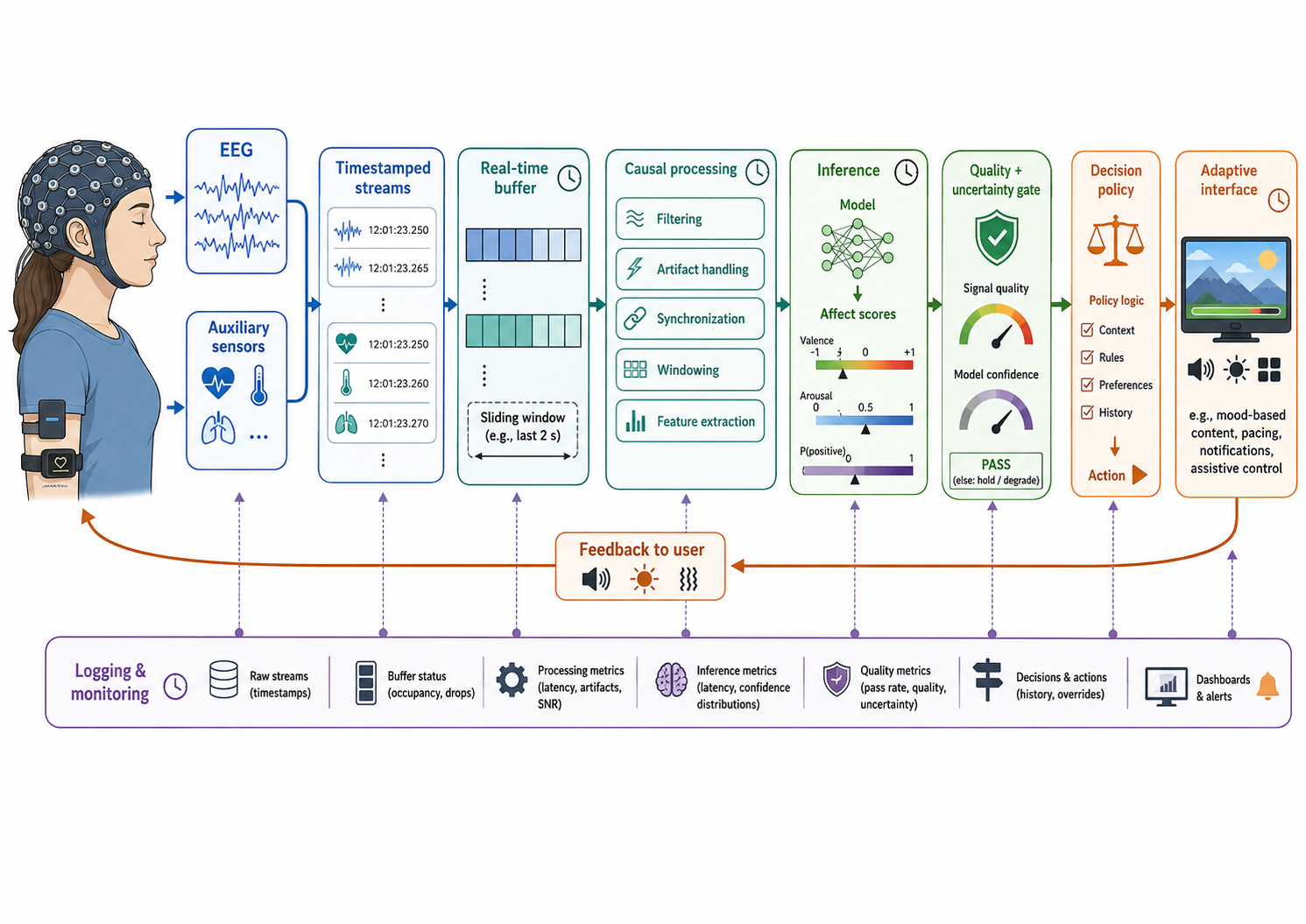
Figure 10.1: End-to-end real-time architecture and latency budget. A live affective BCI is a timed loop from sensors through policy to feedback, with logging beside the loop rather than after it. End-to-end latency is the sum of stage delays, not the model's forward-pass time.
Several Clocks, Not One Time
A sample does not have a single time. At least six distinct times matter:
| Time | Meaning | Typical source of error |
|---|---|---|
| Physiological or event time | When the neural or behavioral event of interest occurred | Unknown; estimated from other timestamps |
| Device timestamp | Clock reading attached at or near digitization | Device clock offset, drift, chunking |
| Arrival time | When software first received the sample | Transport delay, scheduling, USB or wireless buffering |
| Processing time | When preprocessing and inference completed | Queueing, load, garbage collection |
| Decision time | The instant the system commits to a prediction or action | Policy delay after inference |
| Actuation or feedback time | When the user-perceivable output began | Display, audio, or device output latency |
A causal claim at decision time may use only information whose availability is at or before . Availability is not the same as the physiological time the sample describes. Write the associated clocks as
for device, arrival, processing, decision, and feedback time. A sample that describes neural activity at 12.000 s but arrives at 12.040 s is not available at 12.010 s, regardless of its device timestamp.
Clock synchronization and clock drift are therefore first-class engineering problems. Two streams that share a start button can still diverge by tens of milliseconds within minutes if their clocks are independent. Hardware triggers (TTL pulses, a shared analog channel, a dedicated radio-frequency trigger) can align events to a common electrical edge. Software synchronization, including LSL's NTP-style offset estimation between peers, can keep independently clocked streams on a common timeline without dedicated timing hardware. Neither method is universally exact. Hardware triggers do not timestamp every EEG sample, and they do not correct on-device buffering before the pulse is issued. LSL can account for network delay and clock drift between peers, but it cannot observe the throughput delay inside an amplifier or wireless headset: the interval between analog capture and the moment the sample reaches the CPU or microcontroller running the LSL outlet. That on-device delay must be measured, or at least bounded and declared, for each acquisition chain. Treating a software timestamp as physiological time is a specification error, not a rounding error.
Multimodal alignment inherits every one of these issues. Affective systems often combine EEG with video, ratings, physiology, or application logs. Each modality may sample at a different rate, with a different jitter, and with a different device delay. Alignment should be documented as a procedure with residual uncertainty, not as an implicit assumption that "the streams were synced."
Buffers, Continuity, and Broken Streams
Online processing is timestamp-aware. A ring buffer indexed by device or synchronized time, not only by arrival order, is the usual primitive. It has a finite capacity samples or seconds. If production outruns consumption, the oldest samples are overwritten: that is buffer overflow, and it is a data-loss event, not a performance optimization. If consumption outruns production, the policy must wait, abstain, or use a stale window; silently repeating the last sample fabricates continuity.
Late, duplicated, missing, and out-of-order samples are normal in networked and wireless acquisition. A practical inlet should:
- reject or mark duplicates by timestamp or sequence number;
- insert an explicit gap, not interpolated neural data, when a timestamp jump exceeds a declared tolerance;
- reorder within a small jitter window if the transport does not preserve order, then freeze the window once the decision deadline has passed;
- and treat reconnection after dropout as a new continuity epoch, with filter state reset or explicitly carried and logged.
Sampling-rate mismatch requires resampling with an anti-alias filter. Online resampling must itself be causal. A polyphase resampler with a noncausal kernel, or a Fourier interpolator over a future-looking block, is an offline tool. Channel dropout and device reconnection are not equivalent to a missing value in a matrix. A dropped channel may be marked, interpolated from neighbors only if the montage and protocol allow it, or used to enter a degraded state. After reconnection, impedance, reference, and spatial filters may no longer match the calibration session.
Latency, Jitter, Throughput, and Update Rate
Latency should be decomposed rather than advertised as a single number. A compact budget is
where:
- is the delay from analog event to a timestamped sample available in software, including analog filtering, digitization, device buffering, and transport;
- is the wait until a complete causal window of length is present, plus any additional jitter-smoothing wait;
- is causal filtering, resampling, and feature computation after the window is closed;
- is model forward-pass time at batch size one under the deployed hardware load;
- is hysteresis, dwell, confirmation, or other decision delay after scores exist;
- is rendering, audio, haptics, or application-side actuation after the policy commits.
These terms are not interchangeable.
Algorithmic delay is imposed by the mathematics of the estimator: a causal window of seconds cannot report a state whose defining evidence has not yet entered the window. A linear-phase FIR filter of order at sampling rate has group delay
seconds, even before any queueing occurs. That delay is a property of the estimator, not of the computer.
Computational latency is the wall-clock time spent in preprocessing, inference, and policy after the necessary samples have arrived. It depends on CPU or GPU load, memory, thermal throttling, and competing processes. Offline throughput—windows per second on a shuffled dataset with a large batch—does not bound this quantity.
Feedback latency is the additional delay until the user can perceive the result. A prediction completed at that appears on screen 80 ms later has not been delivered at .
Jitter is the variability of these delays. Throughput is the sustained rate at which samples or decisions can be processed without growing queues. Update rate is how often a new decision is issued, typically the reciprocal of the window stride if the pipeline keeps up. A system can have a high update rate and still be late on every decision if exceeds the stride and queues grow.
Latency should be reported as a distribution: at least a median, an upper quantile such as the 95th or 99th percentile, and a worst credible case under declared load, not only a mean. Means hide the stalls that users experience and that closed-loop control cannot ignore.
No single threshold is appropriate for every affective application. A mood estimate updated every few tens of seconds can tolerate a larger than an arousal tracker used to time a breathing cue, which in turn can tolerate more delay than a workload detector that must suppress an interruption before the interruption appears. The latency budget is part of the prediction contract from Chapter 4, not an afterthought attached to a trained model.
Practical Recommendations
- Timestamp at the earliest trusted clock, retain arrival time, and never overwrite one with the other.
- Measure or bound on-device throughput delay; do not treat software synchronization as a substitute for that measurement.
- Size ring buffers from the lookback horizon , the maximum expected jitter, and a declared overflow policy.
- Log gaps, duplicates, reconnects, and clock-offset estimates as first-class events.
- Report as a distribution under the deployed hardware and a specified competing load.
Next: Causal Online Signal Processing and Inference
References
- Schalk, G., McFarland, D. J., Hinterberger, T., Birbaumer, N., and Wolpaw, J. R. (2004). BCI2000: A general-purpose brain-computer interface (BCI) system. IEEE Transactions on Biomedical Engineering, 51(6), 1034-1043.
- Kothe, C., Shirazi, S. Y., Stenner, T., Medine, D., Boulay, C., Grivich, M. I., Artoni, F., Mullen, T., Delorme, A., and Makeig, S. (2025). The lab streaming layer for synchronized multimodal recording. Imaging Neuroscience, 3, IMAG.a.136.
- Pernet, C. R., Appelhoff, S., Gorgolewski, K. J., Flandin, G., Phillips, C., Delorme, A., and Oostenveld, R. (2019). EEG-BIDS, an extension to the BIDS specification for EEG. Scientific Data, 6, 103.
- Zander, T. O., and Kothe, C. (2011). Towards passive brain-computer interfaces: applying brain-computer interface technology to human-machine systems in general. Journal of Neural Engineering, 8(2), 025005.
- Fairclough, S. H. (2009). Fundamentals of physiological computing. Interacting with Computers, 21(1-2), 133-145.