Hybrid Architectures and Advanced Models
Overview
Advanced EEG-based affective computing often requires combining multiple architectural paradigms. Rather than choosing a single architecture (MLP, CNN, LSTM, or Transformer), hybrid models leverage the strengths of different approaches:
- CNNs for automatic spatial-temporal feature extraction
- RNNs/LSTMs for sequential modeling
- Attention/Transformers for global context
- Ensemble methods for robustness
This section explores practical hybrid architectures that achieve state-of-the-art performance on EEG affective computing tasks.
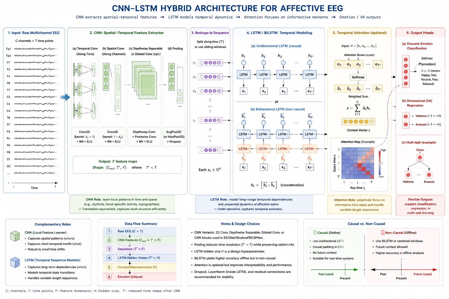
Figure 8.5: CNN-LSTM hybrid architecture for affective EEG. A convolutional front end extracts local spatial-temporal features, while a recurrent back end models their evolution before an affective readout.
CNN-LSTM Hybrid Architecture
Motivation
Combining CNNs and LSTMs offers:
- CNN strength: Automatic feature learning from raw signals
- LSTM strength: Sequential temporal dynamics modeling
Typical pipeline:
Raw EEG
  ↓
CNN: Extract spatial-temporal features (reduce dimensionality)
  ↓
LSTM: Model emotion evolution sequences
  ↓
Emotion prediction
Architecture Design
Variant 1: CNN Feature Extractor + LSTM Classifier
Input: (sequence_length, n_channels)
Example: (2048, 14)
   ↓
[CNN Block]
  Conv1D(64, 32) → ReLU → MaxPool(4)
  Conv1D(128, 16) → ReLU → MaxPool(4)
  Output shape: (128, 256)  # 128 samples, 256 features
   ↓
[LSTM]
  LSTM(64) processes 128 time steps
  Output shape: (64,)
   ↓
[Classification]
  Dense(32) → ReLU → Dense(num_emotions)
Implementation:
from tensorflow.keras import Sequential, layers

model = Sequential([
    layers.Input(shape=(2048, 14)),

    # CNN feature extractor
    layers.Conv1D(64, kernel_size=32, padding='same'),
    layers.ReLU(),
    layers.MaxPooling1D(pool_size=4),
    layers.Dropout(0.3),

    layers.Conv1D(128, kernel_size=16, padding='same'),
    layers.ReLU(),
    layers.MaxPooling1D(pool_size=4),
    layers.Dropout(0.3),

    # LSTM for temporal modeling
    layers.LSTM(64),
    layers.Dropout(0.3),

    # Classification
    layers.Dense(32, activation='relu'),
    layers.Dropout(0.3),
    layers.Dense(3, activation='softmax')  # 3 emotions
])

model.compile(optimizer='adam', loss='categorical_crossentropy', metrics=['accuracy'])
Variant 2: Multi-Scale CNN + Bidirectional LSTM
Captures patterns at different time scales:
Input: (sequence_length, n_channels)
   ↓
[Fast Path]               [Slow Path]
Conv1D(32, kernel=8)      Conv1D(32, kernel=32)
MaxPool(2)                MaxPool(4)
   ↓                         ↓
Concatenate
   ↓
Bidirectional LSTM(64)
   ↓
Output
Variant 3: Channel-Wise CNN + LSTM
Process each channel with separate CNNs, then combine:
Input: (sequence_length, n_channels)
   ↓
[For each channel]
  Conv1D(64, kernel=16) → ReLU → MaxPool(4)
   ↓
Concatenate across channels
Shape: (64, n_channels × 256)
   ↓
LSTM(128)
   ↓
Output
Preprocessing for CNN-LSTM
# 1. Load raw EEG
signal = load_eeg_signal()  # (14, 250000)

# 2. Filter
signal = bandpass_filter(signal, 0.5, 40)

# 3. Create segments
segments = segment_signal(signal, window=2048, overlap=0.5)

# 4. Normalize
segments = (segments - segments.mean()) / segments.std()

# 5. Train
model.fit(segments, labels, epochs=100, batch_size=32)
CNN-Attention Hybrid (Attention-CNN)
Motivation
Add attention mechanisms to CNNs to focus on important time steps and channels.
Architecture
Input: (sequence_length, n_channels)
   ↓
[CNN Feature Extraction]
  Conv1D(64, 32) → ReLU → MaxPool(4)
  Conv1D(128, 16) → ReLU → MaxPool(4)
  Shape: (128, 256)
   ↓
[Channel Attention]
  Compute importance weights for each of 256 features
  Reshape to highlight important features
   ↓
[Temporal Attention]
  Weight importance of each 128 time steps
  Produce context vector
   ↓
[Classification]
  Dense(32) → ReLU → Dense(num_emotions)
Attention Mechanism
Channel Attention:
# For each feature channel:
# 1. Global average pooling: (256,) → scalar for each
# 2. Dense layers to compute attention: scalar → 1 (importance weight)
# 3. Sigmoid to normalize

channel_attention = Sequential([
    layers.GlobalAveragePooling1D(),
    layers.Dense(256 // 16, activation='relu'),
    layers.Dense(256, activation='sigmoid')
])
Temporal Attention:
# For each time step:
# 1. Compute relevance score using query-key mechanism
# 2. Normalize scores with softmax

temporal_attention = Sequential([
    layers.Dense(64, activation='relu'),  # Query
    layers.Dense(1, activation='softmax', bias=False)  # Importance
])
Multi-Task Learning (MTL) Architecture
Motivation
Jointly predict multiple emotional dimensions (valence, arousal, dominance) or auxiliary tasks (action unit detection, facial expression).
Architecture
Input: (sequence_length, n_channels)
   ↓
[Shared Feature Extractor]
  Conv1D + LSTM blocks
  Output: (128,)  shared representation
   ↓
[Task 1: Valence]        [Task 2: Arousal]      [Task 3: Dominance]
Dense(32) → ReLU         Dense(32) → ReLU       Dense(32) → ReLU
Dense(1, Linear)         Dense(1, Linear)       Dense(1, Linear)
MSE loss                 MSE loss               MSE loss
   ↓
Total Loss = α L₁ + β L₂ + γ L₃
Benefits:
- Shared representations learn more robust features
- Reduces overfitting by regularizing shared layers
- Leverages relationships between tasks
- Single model predicts multiple outputs
Implementation
from tensorflow.keras import Model, layers, Input

# Input
input_eeg = Input(shape=(2048, 14))

# Shared feature extraction
x = layers.Conv1D(64, 32, padding='same', activation='relu')(input_eeg)
x = layers.MaxPooling1D(4)(x)
x = layers.LSTM(64)(x)
shared = layers.Dense(128, activation='relu')(x)

# Task-specific heads
valence_out = layers.Dense(32, activation='relu')(shared)
valence_out = layers.Dense(1, name='valence')(valence_out)

arousal_out = layers.Dense(32, activation='relu')(shared)
arousal_out = layers.Dense(1, name='arousal')(arousal_out)

dominance_out = layers.Dense(32, activation='relu')(shared)
dominance_out = layers.Dense(1, name='dominance')(dominance_out)

# Build model
model = Model(inputs=input_eeg, outputs=[valence_out, arousal_out, dominance_out])

model.compile(
    optimizer='adam',
    loss={'valence': 'mse', 'arousal': 'mse', 'dominance': 'mse'},
    loss_weights={'valence': 1.0, 'arousal': 1.0, 'dominance': 0.5}
)

# Train with multiple outputs
model.fit(
    X,
    {'valence': y_valence, 'arousal': y_arousal, 'dominance': y_dominance},
    epochs=100
)
Cross-Modal Fusion Architecture
Scenario
Combining EEG with other modalities: ECG (heart rate), GSR (skin conductance), facial video.
Fusion Strategies
Early Fusion
EEG branch          ECG branch          Video branch
    ↓                  ↓                    ↓
  CNN               Feature Extractor    CNN
    ↓                  ↓                    ↓
Concatenate all features
    ↓
Dense layers
    ↓
Emotion prediction
Pros: Learn interactions between modalities Cons: Requires modalities at same time resolution
Late Fusion
EEG branch          ECG branch          Video branch
    ↓                  ↓                    ↓
  CNN               MLP                 CNN
  Dense(64)        Dense(64)           Dense(64)
    ↓                  ↓                    ↓
Feature vectors from each modality
    ↓
Concatenate
    ↓
Dense layers
    ↓
Emotion prediction
Pros: Each modality learned independently, handles different time rates Cons: May miss fine-grained interactions
Hierarchical Fusion
[Modality-specific fusion at multiple levels]

Level 1: Early stage fusion of some modalities
Level 2: Feature-level fusion
Level 3: Decision-level fusion
Domain Adaptation and Transfer Learning
Challenge
EEG affective models trained on one group often don't generalize to:
- Different subjects (inter-subject variability)
- Different sessions (non-stationarity)
- Different emotion induction methods
- Different datasets
Solution: Domain Adversarial Training
Input: EEG from source domain (training set) and target domain (test set)
   ↓
[Feature Extractor]
  CNN + LSTM layers
  Output: feature representation
   ↓
[Task Classifier]              [Domain Classifier]
Predict emotion               Predict domain (source vs target)
   ↓                            ↓
Classification loss          Adversarial loss
Minimize this                Maximize this (to fool)
Objective: Learn features that are good for emotion prediction but invariant to domain.
Implementation Insight
# During training:
# 1. Compute task loss (emotion classification)
# 2. Compute domain loss (domain adversarial)
# 3. Update feature extractor to minimize task loss
#    but maximize domain loss (via gradient reversal)

loss_total = loss_task - λ × loss_domain
Ensemble Methods
Motivation
Combine predictions from multiple models to improve robustness and reduce overfitting.
Voting Ensemble
models = [
    create_cnn_model(),
    create_lstm_model(),
    create_transformer_model(),
    create_mlp_model()
]

# During prediction:
predictions = [model.predict(X) for model in models]

# Voting:
ensemble_prediction = np.mean(predictions, axis=0)  # Average
# or
ensemble_prediction = np.argmax(np.bincount(predictions))  # Majority vote
Boosting Strategy
# Iteratively train models on harder samples

for iteration in range(n_models):
    # Train model on weighted dataset
    sample_weights = compute_sample_weights(previous_errors)
    model.fit(X, y, sample_weight=sample_weights)

    # Compute errors
    predictions = model.predict(X)
    errors = compute_errors(predictions, y)

    # Increase weights on misclassified samples
    sample_weights[errors > threshold] *= α
Stacking Ensemble
[Meta-features from base models]
  Model 1 prediction
  Model 2 prediction
  Model 3 prediction
    ↓
[Meta-learner]
  Learns how to combine base predictions
    ↓
Final prediction
Recent Advances and Emerging Architectures
Graph Neural Networks (GNNs) for EEG
Represent EEG channel relationships as a graph:
Nodes: EEG channels (electrodes)
Edges: Functional or anatomical connectivity
   ↓
GNN learns patterns in spatial relationships
   ↓
Combines spatial connectivity with emotional dynamics
Advantage: Explicitly models brain network structure Challenge: Limited labeled data for GNN training
See Graph Neural Networks section for comprehensive coverage.
Temporal Convolution Networks (TCNs)
Alternative to RNNs using causal convolutions:
Input: (sequence_length, n_channels)
   ↓
[Dilated Causal Convolutions]
  Convolutions with increasing dilation rates
  Capture multi-scale temporal patterns
   ↓
Output
Advantages: Parallelizable (like Transformers), stable gradients Disadvantage: Fixed receptive field
Vision Transformer (ViT) Variants
Apply Vision Transformer ideas to EEG spectrograms:
Input: Spectrogram (n_freq, n_time)
   ↓
Patch embedding (divide into 16×16 patches)
   ↓
Transformer encoder
   ↓
Emotion classification
Benefit: Leverages large-scale vision pre-training
Selecting the Right Architecture
Decision Framework
Dataset Size?
├─ Small (<500 samples)
│  └─→ MLP with hand-crafted features
│      OR simple CNN with regularization
│
├─ Medium (500-2000 samples)
│  └─→ CNN-LSTM hybrid
│      OR attention-CNN
│
├─ Large (2000-5000 samples)
│  └─→ Deep CNN
│      OR CNN-LSTM
│      OR shallow Transformer
│
└─ Very Large (5000+ samples)
   └─→ Deep Transformer
       OR ensemble hybrid

Computational Resources?
├─ Limited
│  └─→ Avoid Transformer, prefer CNN
│
├─ Moderate
│  └─→ CNN-LSTM hybrid, shallow Transformer
│
└─ Abundant
   └─→ Any architecture, consider ensembles

Real-time Requirement?
├─ Yes, strict latency
│  └─→ MLP, CNN
│
├─ Moderate latency acceptable
│  └─→ CNN-LSTM
│
└─ Offline processing
   └─→ Any architecture
Benchmark Recommendations
| Architecture | Data Size | Speed | Performance | Complexity |
|---|---|---|---|---|
| MLP | Any | ⭐⭐⭐ | ⭐⭐ | ⭐ |
| CNN | 500+ | ⭐⭐ | ⭐⭐⭐ | ⭐⭐ |
| LSTM | 1000+ | ⭐ | ⭐⭐⭐ | ⭐⭐⭐ |
| Transformer | 5000+ | ⭐⭐ | ⭐⭐⭐⭐ | ⭐⭐⭐⭐ |
| CNN-LSTM | 1000+ | ⭐⭐ | ⭐⭐⭐⭐ | ⭐⭐⭐ |
| Attention-CNN | 1000+ | ⭐⭐ | ⭐⭐⭐⭐ | ⭐⭐⭐ |
| Ensemble | Varies | ⭐ | ⭐⭐⭐⭐⭐ | ⭐⭐⭐⭐ |
Best Practices for Hybrid Models
Design Principles
- Balance complexity with data: More parameters need more data
- Component independence: Ensure different components learn different aspects
- Regularization: Critical for hybrid models prone to overfitting
- Interpretability: Understand which components contribute to predictions
- Modularity: Allow easy substitution of components
Training Strategies
- Layer-wise pre-training: Train components separately, then jointly
- Curriculum learning: Start with simpler tasks, progress to complex
- Joint training: All components from scratch, balanced loss weights
- Alternating optimization: Train components sequentially
Validation and Evaluation
- Cross-validation: Standard k-fold insufficient for temporal data
- Leave-one-subject-out: Critical for inter-subject generalization
- Leave-one-session-out: Tests within-subject generalization
- Ablation studies: Remove components to assess contribution
- Attention visualization: Understand model's focus
Practical Implementation Considerations
Computational Cost
# Estimate memory usage
batch_size = 32
seq_len = 2048
n_channels = 14

# CNN
param_cnn = 64 * 32 + 128 * 16  # Rough estimate
memory_cnn = batch_size * seq_len * n_channels * 4 / 1e6  # MB

# LSTM (hidden states)
memory_lstm = batch_size * seq_len * 64 * 4 / 1e6  # MB

# Combined
total = memory_cnn + memory_lstm  # Add overhead
Hyperparameter Tuning
Use grid or random search:
hyperparams = {
    'n_conv_filters': [32, 64, 128],
    'lstm_units': [32, 64, 128],
    'dropout': [0.2, 0.3, 0.5],
    'learning_rate': [0.001, 0.0001]
}

# Grid search over combinations
Summary
Hybrid architectures represent the current state-of-the-art for EEG-based affective computing:
Key Advantages:
- Combine strengths of different paradigms
- Better generalization across subjects/sessions
- More robust to noise and variability
- Can leverage multiple complementary information sources
Practical Recommendations:
- Start with CNN-LSTM for moderate datasets and balanced performance
- Use attention mechanisms to improve interpretability
- Apply multi-task learning when multiple emotion dimensions available
- Consider ensembles for critical applications
- Use domain adaptation for cross-dataset generalization
Future Directions:
- Increasingly leveraging pre-trained models and transfer learning
- Incorporating domain knowledge (e.g., frequency bands)
- Explainable AI for clinical applicability
- Efficient architectures for edge deployment
Conclusion: Deep learning offers powerful tools for EEG-based affective computing. Success requires matching architecture complexity to available data, carefully designing inputs and preprocessing, and validating across subjects and sessions. Hybrid approaches and ensemble methods typically provide the best balance of performance and robustness.
Next: Graph Neural Networks
References
- Caruana, R. (1997). Multitask learning. Machine Learning, 28, 41–75.
- Ganin, Y., Ustinova, E., Ajakan, H., et al. (2016). Domain-adversarial training of neural networks. JMLR, 17(59), 1–35.
- Baltrušaitis, T., Ahuja, C., and Morency, L.-P. (2019). Multimodal machine learning: A survey and taxonomy. IEEE Transactions on Pattern Analysis and Machine Intelligence, 41(2), 423–443.
- Bai, S., Kolter, J. Z., and Koltun, V. (2018). An empirical evaluation of generic convolutional and recurrent networks for sequence modeling. arXiv:1803.01271.
- Ding, Y., Robinson, N., Zhang, S., Zeng, Q., and Guan, C. (2022). TSception: Capturing temporal dynamics and spatial asymmetry from EEG for emotion recognition. IEEE Transactions on Affective Computing, 13(4), 2232–2245.