Neural Operator Learning for Affective EEG
Most neural networks learn a finite-dimensional map: a fixed-size EEG tensor enters, and a label or another fixed-size tensor leaves. Neural operators instead learn mappings between functions. Their target is an operator that can act on a signal sampled at different temporal resolutions, spatial grids, or sensor layouts. This perspective is attractive for EEG because recordings are continuous in time, differ in sampling rate and montage, and often need to be modeled as fields rather than as one fixed vector shape.
Neural operators do not replace CNNs, Transformers, or GNNs for every affective task. They are most compelling when the input-output relation is naturally functional: reconstruction of missing channels, continuous signal transformation, cross-device translation, neural-field modeling, or learning dynamics that should transfer across resolutions.
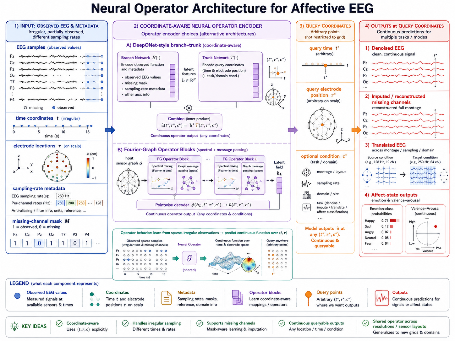
Figure 8.12: Neural operator architecture for affective EEG. Coordinate-aware neural operators map sampled EEG functions to continuous outputs at requested times, electrode locations, or resolutions rather than assuming one fixed input grid.
Operator Learning Intuition
Let be an input function, such as a multichannel EEG signal over time and electrode location, and let be an output function. A neural operator learns
Unlike a standard network tied to one discretization, the goal is to approximate across sampled versions of the underlying function. For EEG, can denote signal value at time and electrode or source location . The output may be a denoised signal, an imputed channel field, a latent neural field, a future trajectory, or a continuous affect-state field.
In practice, discretization invariance is approximate, not automatic. A model still needs explicit handling of sampling rates, channel coordinates, reference schemes, and missing sensors. Claims of resolution or montage transfer should be tested directly rather than assumed from the operator formulation.
Core Neural Operator Families
| Family | Main idea | EEG-relevant strength | Main limitation |
|---|---|---|---|
| DeepONet | Branch network encodes sampled input; trunk network encodes query coordinates | Predict values at arbitrary times or sensor locations | Query design and training coverage are critical |
| Fourier Neural Operator (FNO) | Learns global updates in Fourier space | Efficient long-range temporal and spectral interactions | Standard FNO assumes regular grids and can be sensitive to nonstationarity |
| Wavelet Neural Operator | Uses localized multiscale wavelet representations | Better localization of transient EEG events | More design choices and less mature tooling |
| Graph Neural Operator | Replaces regular-grid kernels with graph-based integral operators | Handles irregular electrode montages and source graphs | Depends on graph quality and may be expensive |
| Geometry-aware operator | Conditions on coordinates or manifold geometry | Supports sensor locations and subject-specific head geometry | Requires reliable coordinate and geometry metadata |
DeepONet
DeepONet represents an operator using a branch network that reads sampled input values and a trunk network that reads an output query coordinate. A simplified form is
where is the branch representation of the input function and is the trunk representation of coordinate . For EEG, can encode time, electrode position, source location, frequency, or a combination of these.
Example scenario: A DeepONet receives a subset of wearable EEG channels and queries the trunk at missing electrode coordinates. It predicts a continuous approximation of those missing channels, with the sensor coordinates and montage supplied explicitly. Evaluation measures reconstruction on held-out real channels and downstream affect performance, not only training reconstruction error.
Fourier Neural Operator
FNO layers mix local features with global spectral convolution. A typical update is
where is a Fourier transform and learns weights for retained modes. For EEG, Fourier mixing can model long-range temporal dependencies and spectral structure efficiently, especially for long stationary or quasi-stationary segments.
However, EEG has transient events, nonstationarity, artifacts, and irregular electrode layouts. Practical variants may use short-time Fourier patches, separate temporal and spatial operator blocks, adaptive mode selection, or wavelet-style local representations rather than one global transform over an entire recording.
Graph and Geometry Integration
Electrodes are irregularly placed sensors, so a regular temporal grid alone is insufficient for many EEG applications. Graph neural operators define an operator on nodes and edges, often using an integral-kernel or message-passing form:
where and can include electrode coordinates, features, or source locations and encodes edge information. The graph can represent physical electrode distance, a head-surface mesh, anatomical adjacency, functional connectivity, or a causal graph; each choice supports a different claim.
Promising EEG integrations include:
- a temporal FNO followed by a graph operator over electrodes;
- a graph neural operator that conditions kernels on electrode coordinates and head geometry;
- source-space operators over cortical meshes;
- dynamic graph operators with connectivity estimated per time interval;
- and neural operators constrained by a stable directed graph when causal modeling assumptions are justified.
A graph operator should preserve channel identity and missing-channel masks. It should not treat an absent electrode as a zero-valued measurement without a documented policy.
Applications to Affective EEG
Neural operators are most plausible when the output has functional structure:
- Denoising and artifact correction: Map noisy continuous EEG to a cleaned signal while preserving event timing and spectra.
- Missing-channel imputation: Predict sensor or source values at unobserved spatial coordinates.
- Cross-montage translation: Map a low-density wearable montage to a representation compatible with a higher-density model, with uncertainty estimates.
- Continuous affect fields: Map EEG streams to continuous valence-arousal trajectories rather than isolated labels.
- Dynamics modeling: Learn an operator that evolves latent neural or affective fields over time.
- Surrogate forward models: Approximate computationally expensive mappings in source imaging or biophysical simulations.
For ordinary trial-level classification on a fixed 32-channel montage, a CNN, Transformer, or GNN is usually a simpler and stronger baseline. Operator learning earns its complexity when discretization, spatial querying, or continuous outputs are part of the scientific requirement.
Recent Directions and Variations
Several developments are relevant to EEG research:
- Multi-resolution and wavelet operators improve localization of brief transients and cross-scale rhythms.
- Factorized and low-rank operators reduce computation for long sequences and many channels.
- Physics-informed neural operators add constraints from known forward models, signal propagation, or dynamical priors.
- Operator transformers use attention to learn query-dependent global interactions while retaining coordinate-aware outputs.
- Uncertainty-aware operators estimate epistemic and observation uncertainty for missing channels, artifacts, or out-of-distribution montages.
- Foundation-style operator pretraining can learn broad continuous signal transformations before low-label affect adaptation, provided pretraining/evaluation splits prevent subject and dataset leakage.
These directions remain early for affective EEG. Strong empirical work should compare them with resolution-matched baselines and explain why an operator, rather than a conventional architecture, matches the task.
Training and Evaluation
Train using source-level grouping so that windows from one recording do not leak across partitions. If a model claims resolution transfer, hold out sampling rates, query points, channels, montages, or subjects in a way that directly tests that claim. Fit all normalization and coordinate transforms on training data only.
Evaluate at multiple levels:
| Claim | Evaluation |
|---|---|
| Signal reconstruction | Time-domain error, spectral error, phase-sensitive measures, artifact preservation checks |
| Spatial query or imputation | Held-out channel reconstruction across subjects and montages |
| Resolution transfer | Train and test at different temporal sampling or query resolutions |
| Downstream affect utility | Train or evaluate affect decoder on untouched real held-out recordings |
| Robustness | Missing channels, sensor noise, montage mismatch, and temporal nonstationarity |
| Efficiency | Memory, latency, and scaling with sequence length and channel count |
Visual plausibility is not sufficient. Generated or reconstructed EEG should preserve relevant spectra, channel relationships, timing, and downstream task behavior on real held-out data.
Practical Recommendations
- Begin with a fixed-grid CNN, Transformer, or GNN baseline before adopting an operator.
- Encode time, electrode coordinates, channel masks, and sampling information explicitly.
- Use FNO-style methods for long regular temporal fields; use graph or geometry-aware operators for irregular montages.
- Prefer wavelet or multiresolution variants when transient events and nonstationarity are central.
- Report discretization, coordinate system, retained modes, query scheme, and cross-resolution evaluation protocol.
- Keep claims modest: resolution transfer and interpolation are empirical properties, not guarantees of the architecture.
References
- Lu, L., Jin, P., Pang, G., Zhang, Z., and Karniadakis, G. E. (2021). Learning nonlinear operators via DeepONet based on the universal approximation theorem of operators. Nature Machine Intelligence, 3, 218-229.
- Li, Z., Kovachki, N., Azizzadenesheli, K., et al. (2021). Fourier neural operator for parametric partial differential equations. International Conference on Learning Representations.
- Kovachki, N., et al. (2023). Neural operator: Learning maps between function spaces with applications to PDEs. Journal of Machine Learning Research, 24, 1-97.
- Li, Z., Huang, D. Z., Liu, B., and Anandkumar, A. (2020). Fourier neural operator with learned deformations for PDEs on general geometries. arXiv:2010.08895.
- Li, Z., Kovachki, N., Azizzadenesheli, K., et al. (2020). Neural operator: Graph kernel network for partial differential equations. arXiv:2003.03485.