Generative Adversarial Networks (GANs) for EEG
Overview
Generative Adversarial Networks frame generation as a competitive game between two networks: a generator that creates synthetic EEG and a discriminator that distinguishes real from fake. Through adversarial training, the generator learns to produce increasingly realistic EEG signals. GANs excel at data augmentation, domain adaptation, and artifact removal in EEG-based affective computing.
Generative Adversarial Network Architecture
A generative adversarial network consists of two neural networks trained in opposition: a generator $G$ and a discriminator $D$. The generator maps a random latent vector $z$, sampled from a simple distribution such as a standard Gaussian, to a synthetic observation $G(z)$. The discriminator receives both real training examples and generated examples, and learns to estimate whether each input came from the data distribution or the generator. The generator is updated through the discriminator's feedback so that its synthetic samples become increasingly difficult to distinguish from real data.
Rather than explicitly modeling a likelihood, GANs learn the target distribution through this adversarial game. Training alternates between improving $D$'s real-versus-fake decision and improving $G$'s ability to fool $D$. Once training is complete, only the generator is needed to produce new samples; conditions such as an emotion class or subject identifier can also be supplied to both networks to enable targeted generation. For EEG, this supports the synthesis of multichannel signals with realistic temporal and spectral structure.
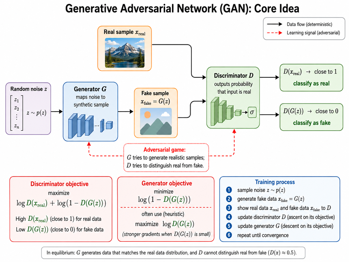
Figure 8.11: Generative adversarial network architecture. The generator converts latent noise into synthetic samples, while the discriminator compares real and generated samples and supplies the adversarial learning signal.
Theoretical Foundations
The Adversarial Game
Generator : Maps random noise to synthetic EEG Discriminator : Classifies input as real () or fake ()
The minimax objective:
Training Dynamics
The two losses should not be read as ordinary accuracy measures: a lower discriminator loss is not automatically better if it leaves the generator with no useful gradient. Healthy training is a moving balance in which the discriminator remains informative and the generator gradually covers diverse real-signal patterns. For EEG, visual plausibility alone is insufficient; the game must also preserve band power, temporal structure, and relationships between channels.
For each iteration:
  1. Train D: maximize ability to distinguish real from fake
  2. Train G: maximize D's error (generate more realistic samples)
  3. Repeat until Nash equilibrium
Why GANs for EEG?
Advantages:
- Sharp generations: Unlike VAEs, GANs produce crisp, high-frequency details
- No explicit likelihood: Learns data distribution implicitly (more flexible)
- Domain translation: CycleGAN enables subject-to-subject EEG translation
- Data augmentation: Generate unlimited synthetic training data
- Artifact removal: Pix2Pix-style conditional GANs for denoising
- Unsupervised feature learning: Discriminator learns useful EEG features
Challenges:
- Training instability (mode collapse, vanishing gradients)
- No encoder (harder to map real EEG to latent space)
- Evaluation difficulty (no likelihood, reliance on FID-like metrics)
- Hyperparameter sensitivity
GAN Architectures for EEG
GAN variants alter the adversarial objective, conditioning mechanism, or transformation task to address different EEG-generation goals (Figure 8.12). DCGAN uses convolutional generator and discriminator networks for direct signal synthesis; CGAN incorporates labels for emotion-controlled generation; WGAN and WGAN-GP replace the original divergence with a Wasserstein objective to improve stability; CycleGAN learns unpaired translation between domains such as subjects or recording sessions; and SRGAN targets signal enhancement or resolution recovery. Selecting a variant should follow the intended EEG task rather than sample realism alone.
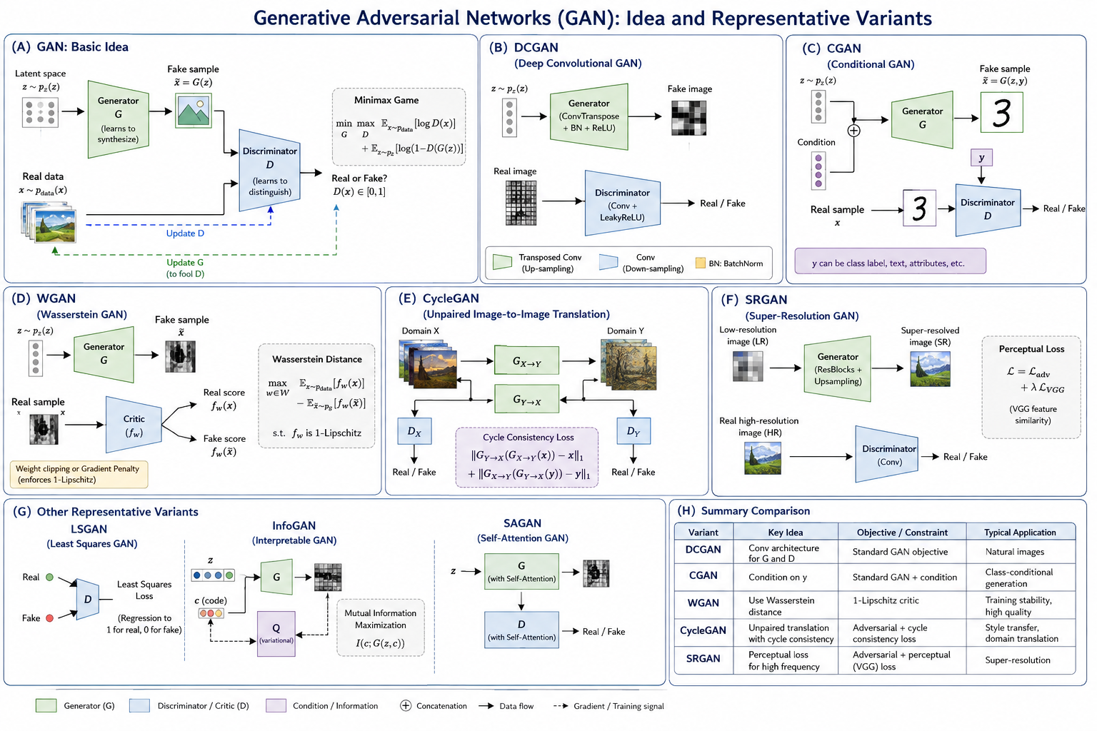
Figure 8.12: GAN variants and their roles in EEG analysis. DCGAN provides convolutional synthesis; CGAN conditions generation on labels; WGAN/WGAN-GP improve adversarial training stability; CycleGAN enables unpaired cross-domain translation; and SRGAN learns to reconstruct higher-resolution signals from lower-resolution inputs.
1. Deep Convolutional GAN (DCGAN)
The foundational GAN architecture adapted for 1D EEG signals:
The generator expands a compact noise vector into a full multichannel time series, while the discriminator progressively compresses a time series into one realism score. Strided convolutions make this tractable for long recordings, but can introduce periodic artifacts or neglect slow rhythms. Kernel sizes, stride, and output scaling should therefore be selected with the sampling rate and EEG bands of interest in mind.
Generator:
  z ~ N(0,I) (latent_dim=100)
    ↓
  Dense(256 × 64) → Reshape(64, 256)
    ↓
  Conv1DTranspose(128, 5, stride=2) → BN → ReLU
    ↓
  Conv1DTranspose(64, 5, stride=2) → BN → ReLU
    ↓
  Conv1DTranspose(32, 5, stride=2) → BN → ReLU
    ↓
  Conv1DTranspose(14, 5, stride=2) → Tanh
    ↓
  Output: (14 channels, 2048 samples)

Discriminator:
  Input: (14 channels, 2048 samples)
    ↓
  Conv1D(32, 5, stride=2) → LeakyReLU(0.2)
    ↓
  Conv1D(64, 5, stride=2) → BN → LeakyReLU(0.2)
    ↓
  Conv1D(128, 5, stride=2) → BN → LeakyReLU(0.2)
    ↓
  Conv1D(256, 5, stride=2) → BN → LeakyReLU(0.2)
    ↓
  Flatten → Dense(1) → Sigmoid
    ↓
  Real (1) or Fake (0)
2. Conditional GAN (CGAN)
Generate EEG conditioned on emotion labels:
Conditioning closes the gap between realistic generation and useful generation. It gives the model a target class, but the discriminator must see the same condition; otherwise the generator can ignore it. Classifier accuracy on generated signals, balanced across labels, is a simple check that the label has affected the signal rather than merely being passed through the API.
Generator:
  z (noise) + y (emotion label)
    ↓
  Generates EEG with specific emotional content

Discriminator:
  x (EEG) + y (emotion label)
    ↓
  Real/fake + correct emotion?
Application: Generate training samples for specific under-represented emotions.
3. Wasserstein GAN (WGAN / WGAN-GP)
Uses Earth Mover's distance for more stable training:
The practical motivation is that the original GAN discriminator can become overconfident when real and generated EEG distributions barely overlap, producing weak gradients for the generator. WGAN replaces probability classification with a critic score, and the gradient penalty encourages the critic to change smoothly between real and generated signals. This is especially valuable for small, heterogeneous EEG datasets, although it increases the cost of each training step.
With gradient penalty (WGAN-GP):
EEG relevance: More stable training is critical for small EEG datasets.
4. CycleGAN for Cross-Subject EEG Translation
Translates EEG from one subject's "style" to another:
Cycle consistency provides a safeguard in the absence of paired recordings: an EEG segment translated from subject A to B and back again should retain its original content. It reduces arbitrary transformations, but does not guarantee that emotion is preserved. When using CycleGAN for subject adaptation, validate the translated output against known labels and ensure the method does not amplify demographic or acquisition-related biases.
Subject A EEG → Generator A→B → Subject B EEG → Discriminator B
                                                    ↓
                                              Real B or Fake B?
Subject B EEG → Generator B→A → Subject A EEG → Discriminator A
                                                    ↓
                                              Real A or Fake A?

+ Cycle consistency: A → B → A ≈ A (preserve emotional content)
Application: Normalize inter-subject variability, enabling better cross-subject generalization.
5. Super-Resolution GAN (SRGAN)
Enhance low-resolution EEG to high-resolution:
Low-res EEG (few channels, low sampling rate)
    ↓
Generator (upsampling network)
    ↓
High-res EEG (many channels, high sampling rate)
    ↓
Discriminator: Real or Fake high-res?
Application: Upgrade consumer-grade EEG (4 channels) to research-grade (64 channels).
Implementation
WGAN-GP for EEG Generation
This implementation separates the generator, critic, and training controller so that the adversarial roles remain clear. The critic is updated several times for each generator update because it must provide a useful transport-distance estimate before the generator moves. The gradient penalty is evaluated on interpolated real and fake samples; its purpose is to regularize the critic, not to make the EEG waveform itself smoother.
import tensorflow as tf
from tensorflow.keras import layers, Model

class EEGGenerator(Model):
    def __init__(self, latent_dim=100):
        super().__init__()
        self.model = tf.keras.Sequential([
            layers.Dense(256 * 64, input_shape=(latent_dim,)),
            layers.Reshape((64, 256)),
            layers.BatchNormalization(),
            layers.ReLU(),

            layers.Conv1DTranspose(128, 5, strides=2, padding='same'),
            layers.BatchNormalization(),
            layers.ReLU(),

            layers.Conv1DTranspose(64, 5, strides=2, padding='same'),
            layers.BatchNormalization(),
            layers.ReLU(),

            layers.Conv1DTranspose(32, 5, strides=2, padding='same'),
            layers.BatchNormalization(),
            layers.ReLU(),

            layers.Conv1DTranspose(14, 5, strides=2, padding='same'),
            layers.Activation('tanh'),
        ])

    def call(self, z):
        return self.model(z)

class EEGDiscriminator(Model):
    def __init__(self):
        super().__init__()
        self.model = tf.keras.Sequential([
            layers.Conv1D(32, 5, strides=2, padding='same',
                         input_shape=(2048, 14)),
            layers.LeakyReLU(0.2),

            layers.Conv1D(64, 5, strides=2, padding='same'),
            layers.LayerNormalization(),
            layers.LeakyReLU(0.2),

            layers.Conv1D(128, 5, strides=2, padding='same'),
            layers.LayerNormalization(),
            layers.LeakyReLU(0.2),

            layers.Conv1D(256, 5, strides=2, padding='same'),
            layers.LayerNormalization(),
            layers.LeakyReLU(0.2),

            layers.Flatten(),
            layers.Dense(1),  # No sigmoid for WGAN
        ])

    def call(self, x):
        return self.model(x)

# WGAN-GP Training
class WGAN_GP(Model):
    def __init__(self, latent_dim=100, gp_weight=10.0):
        super().__init__()
        self.generator = EEGGenerator(latent_dim)
        self.discriminator = EEGDiscriminator()
        self.latent_dim = latent_dim
        self.gp_weight = gp_weight

    def gradient_penalty(self, real, fake):
        """Compute gradient penalty for WGAN-GP"""
        batch_size = tf.shape(real)[0]
        alpha = tf.random.uniform([batch_size, 1, 1], 0.0, 1.0)

        interpolated = alpha * real + (1 - alpha) * fake

        with tf.GradientTape() as tape:
            tape.watch(interpolated)
            d_interpolated = self.discriminator(interpolated)

        gradients = tape.gradient(d_interpolated, [interpolated])[0]
        grad_norm = tf.sqrt(tf.reduce_sum(
            tf.square(gradients), axis=[1, 2]
        ))
        return tf.reduce_mean((grad_norm - 1.0) ** 2)

    def train_step(self, real_eeg):
        batch_size = tf.shape(real_eeg)[0]

        # Train discriminator (multiple steps per generator step)
        for _ in range(5):
            z = tf.random.normal((batch_size, self.latent_dim))

            with tf.GradientTape() as tape:
                fake_eeg = self.generator(z)
                d_real = self.discriminator(real_eeg)
                d_fake = self.discriminator(fake_eeg)

                gp = self.gradient_penalty(real_eeg, fake_eeg)
                d_loss = tf.reduce_mean(d_fake) - tf.reduce_mean(d_real) + self.gp_weight * gp

            d_grads = tape.gradient(d_loss, self.discriminator.trainable_variables)
            self.optimizer.apply_gradients(
                zip(d_grads, self.discriminator.trainable_variables)
            )

        # Train generator
        z = tf.random.normal((batch_size, self.latent_dim))

        with tf.GradientTape() as tape:
            fake_eeg = self.generator(z)
            d_fake = self.discriminator(fake_eeg)
            g_loss = -tf.reduce_mean(d_fake)

        g_grads = tape.gradient(g_loss, self.generator.trainable_variables)
        self.optimizer.apply_gradients(
            zip(g_grads, self.generator.trainable_variables)
        )

        return {'d_loss': d_loss, 'g_loss': g_loss}
CycleGAN for Cross-Subject Translation
Unlike the noise-to-signal WGAN generator above, CycleGAN generators must map one signal directly into another signal of the same shape. The code emphasizes cycle and identity losses because adversarial loss alone would permit a generator to change any aspect of the recording that fools the discriminator. In a full training loop, those losses should be weighted and reported separately to reveal whether translation is preserving content or merely minimizing pixel-level differences.
class CycleGAN_EEG(Model):
    def __init__(self):
        super().__init__()
        # Generators: Subject A ↔ Subject B
        self.G_A2B = EEGGenerator()
        self.G_B2A = EEGGenerator()

        # Discriminators
        self.D_A = EEGDiscriminator()  # Distinguish real A from fake A
        self.D_B = EEGDiscriminator()  # Distinguish real B from fake B

    def cycle_consistency_loss(self, real_A, real_B):
        """Ensure A → B → A ≈ A and B → A → B ≈ B"""
        # Forward cycle: A → B → A
        fake_B = self.G_A2B(real_A)       # Real A to B-style but with A's emotion
        cycle_A = self.G_B2A(fake_B)      # Back to A-style
        loss_cycle_A = tf.reduce_mean(tf.abs(real_A - cycle_A))

        # Backward cycle: B → A → B
        fake_A = self.G_B2A(real_B)
        cycle_B = self.G_A2B(fake_A)
        loss_cycle_B = tf.reduce_mean(tf.abs(real_B - cycle_B))

        return loss_cycle_A + loss_cycle_B

    def identity_loss(self, real_A, real_B):
        """G should preserve content when input already in target domain"""
        id_A = self.G_B2A(real_A)  # A → A (should not change)
        id_B = self.G_A2B(real_B)  # B → B (should not change)

        return (tf.reduce_mean(tf.abs(real_A - id_A)) +
                tf.reduce_mean(tf.abs(real_B - id_B)))

    def call(self, inputs, training=False):
        real_A, real_B = inputs

        fake_B = self.G_A2B(real_A)
        fake_A = self.G_B2A(real_B)

        if training:
            # Compute all losses...
            pass

        return fake_B, fake_A
Applications in EEG Affective Computing
GAN applications should be framed as distribution-learning experiments, not as a licence to manufacture arbitrary EEG. Hold out subjects and sessions before GAN training when the downstream goal is generalization, and compare generated and real signals with PSD, connectivity, channel-correlation, and classifier-based metrics. The central question is whether synthetic data improves a pre-specified downstream task without leaking information from its evaluation set.
1. Data Augmentation for Imbalanced Emotions
Emotion datasets are often imbalanced — GANs can balance them:
# Dataset: 80% neutral, 15% happy, 5% sad
# Problem: Sad class has too few samples

# Train Conditional GAN on all classes
cgan = ConditionalGAN()

# Generate synthetic sad EEG
synthetic_sad = cgan.generate(label='sad', n_samples=500)

# Augmented dataset now has balanced classes
augmented_X = np.concatenate([real_X, synthetic_sad])
augmented_y = np.concatenate([real_y, ['sad'] * 500])

# Train classifier on augmented data → better minority class performance
2. Cross-Subject Domain Adaptation
Reduce inter-subject variability without losing emotional content:
# Source subject: Subject A (well-labeled)
# Target subject: Subject B (few or noisy labels)

# Train CycleGAN: A ↔ B translation
cyclegan = CycleGAN_EEG()
cyclegan.fit(subject_A_eeg, subject_B_eeg)

# Translate A's labeled data to B's "style"
A_translated_to_B = cyclegan.G_A2B(subject_A_eeg)

# Train classifier on translated data
classifier.fit(A_translated_to_B, labels_A)
# Classifier now works on Subject B!
3. Artifact Removal (EEG Denoising)
Train a GAN to clean EEG artifacts:
# Paired training data:
#   Input: Noisy EEG (with eye blinks, muscle artifacts)
#   Target: Clean EEG (artifact removed)

# Pix2Pix-style conditional GAN:
generator = UNet()  # Noisy EEG → Clean EEG
discriminator = PatchGAN()  # Real/fake on patches

# Loss = GAN loss + L1 reconstruction loss
loss = gan_loss(discriminator(clean, generated)) + lambda_l1 * |clean - generated|
4. Cross-Modal EEG Generation
Generate EEG from other modalities:
# Input: Facial expression video features
# Output: Corresponding EEG signals

# This enables:
# - Predicting EEG from easily obtained video
# - Studying video-EEG correspondences
# - Filling missing EEG sessions
5. Style-Based EEG Manipulation
StyleGAN-inspired architecture for controlled EEG editing:
# StyleGAN mapping:
z → Mapping Network → w (style vector)
w → Synthesis Network → EEG

# Manipulate specific "styles":
# - w[0:2]: Emotional valence
# - w[2:4]: Emotional arousal
# - w[4:6]: Subject identity
# - w[6:8]: Noise/artifacts

# Change emotion without changing subject:
w_modified = w.copy()
w_modified[0:2] = new_valence_style
new_eeg = synthesis_network(w_modified)
GAN Training Stability for EEG
EEG signals are challenging for GANs due to high dimensionality and limited data. Strategies:
Most stability techniques address a single failure mode: the discriminator may dominate, the generator may collapse to a few stereotyped trials, or the networks may learn shortcuts based on amplitude and acquisition artifacts. Apply them incrementally and record which change improves both training behavior and EEG-specific validation measures; combining many methods at once makes failures difficult to diagnose.
1. Gradient Penalty (WGAN-GP)
# Most important stabilization technique
gp_loss = lambda * ((grad_norm - 1) ** 2).mean()
2. Spectral Normalization
# Normalize discriminator weights
from tensorflow.keras.layers import Conv1D

class SpectralNormConv1D(Conv1D):
    def build(self, input_shape):
        super().build(input_shape)
        # Apply spectral normalization to kernel
        self.u = self.add_weight(
            name='u', shape=(1, self.filters),
            initializer='random_normal', trainable=False
        )
3. Progressive Growing
# Start with low-resolution EEG (fewer time samples)
# Gradually increase resolution during training
# Stabilizes early training and improves final quality

stages = [
    (512,),     # Stage 1: ~2 seconds
    (1024,),    # Stage 2: ~4 seconds
    (2048,),    # Stage 3: ~8 seconds
]
4. Two Time-Scale Update Rule (TTUR)
# Different learning rates for G and D
g_optimizer = Adam(lr=0.0001, beta_1=0.5)
d_optimizer = Adam(lr=0.0004, beta_1=0.5)  # D learns faster
5. Minibatch Discrimination
# Help GAN capture EEG diversity across subjects
# Discriminator looks at minibatch statistics, not just single samples
Evaluation Metrics for EEG GANs
No one metric establishes that a GAN has learned useful EEG. Distributional scores quantify similarity in a chosen feature space, whereas downstream accuracy tests utility and expert review tests face validity. Report several complementary measures, use the same feature extractor for all comparisons, and include real-versus-real baselines so that the unavoidable variability between genuine recordings is visible.
| Metric | Description | EEG Adaptation |
|---|---|---|
| Inception Score (IS) | Quality + diversity | Need EEG-specific classifier (e.g., EEGNet) |
| FID | Distribution distance | Extract features from EEG classifier |
| Spectral FID | PSD-based distance | Compare frequency content |
| Classification Accuracy Gain | Improvement from augmentation | Train classifier on real+generated data |
| Expert Turing Test | Human expert evaluation | Can neuroscientist distinguish real from generated? |
| Channel Correlation Preservation | Spatial structure preserved? | Compare real vs. generated channel correlation matrices |
Comparison: GAN vs. VAE for EEG
| Aspect | GAN | VAE |
|---|---|---|
| Sample quality | Sharp, realistic (high-freq details) | Smoother, slightly blurry |
| Latent space | None (implicit), harder to encode | Structured (Gaussian), easy to encode |
| Training stability | Can be unstable | Generally stable |
| Mode coverage | Mode collapse risk | Good coverage |
| Data augmentation | Excellent | Good |
| Interpretability | Limited | Better (disentanglement) |
| Interpolation | Possible with StyleGAN-like | Natural (linear in z) |
| EEG realism | Higher PSD fidelity | Better distribution matching |
Best Practices
- Start with WGAN-GP: Most stable variant for EEG
- Normalize carefully: [-1, 1] range for tanh output
- Use spectral normalization on discriminator
- Monitor FID and spectral similarity during training
- Augment training data with traditional methods first (time shift, noise)
- Pre-train discriminator as EEG classifier before GAN training
- Validate neuroscientifically: Check frequency bands in generated EEG
- Combine with VAE: VAE-GAN hybrids leverage both paradigms
Summary
GANs provide a powerful adversarial framework for EEG generation and transformation:
Key Strengths for EEG:
- Generate realistic, sharp EEG samples for data augmentation
- Cross-subject domain adaptation without paired data
- Powerful artifact removal and denoising
- Style-based manipulation for controlled generation
- No explicit distributional assumptions
When to Use GANs:
- Data augmentation for imbalanced emotion datasets
- Cross-subject EEG translation (CycleGAN)
- Artifact removal and signal enhancement
- Need for sharp, high-quality generated samples
- Unsupervised domain adaptation
When to Prefer Alternatives:
- Need structured latent space → VAE
- Need exact likelihood → Flow/Diffusion
- Training instability is a blocker → VAE
- Small datasets (<500 samples) → VAE may generalize better
Next: Flow-based Models and Diffusion Models
References
- Goodfellow, I., Pouget-Abadie, J., Mirza, M., et al. (2014). Generative adversarial nets. In NeurIPS.
- Radford, A., Metz, L., and Chintala, S. (2016). Unsupervised representation learning with deep convolutional generative adversarial networks. In ICLR.
- Mirza, M., and Osindero, S. (2014). Conditional generative adversarial nets. arXiv:1411.1784.
- Arjovsky, M., Chintala, S., and Bottou, L. (2017). Wasserstein generative adversarial networks. In ICML.
- Gulrajani, I., Ahmed, F., Arjovsky, M., Dumoulin, V., and Courville, A. (2017). Improved training of Wasserstein GANs. In NeurIPS.
- Zhu, J.-Y., Park, T., Isola, P., and Efros, A. A. (2017). Unpaired image-to-image translation using cycle-consistent adversarial networks. In ICCV.
- Miyato, T., Kataoka, T., Koyama, M., and Yoshida, Y. (2018). Spectral normalization for generative adversarial networks. In ICLR.
- Karras, T., Aila, T., Laine, S., and Lehtinen, J. (2018). Progressive growing of GANs for improved quality, stability, and variation. In ICLR.