Transformer Models for EEG-based Affective Computing
Overview
Transformer models revolutionized deep learning by replacing recurrent mechanisms with attention mechanisms. Unlike RNNs that process sequences sequentially, Transformers process all time steps in parallel, enabling efficient training on long sequences. Recent advances have made Transformers increasingly popular for EEG analysis, offering both computational efficiency and strong performance.
Transformer Architecture
A Transformer turns an input sequence into a sequence of tokens, each represented by a learned embedding vector. Because attention alone has no notion of order, positional information is added to every token. The resulting token sequence passes through a stack of Transformer blocks. Each block first uses multi-head self-attention to let every token exchange information with other tokens, then applies a feed-forward network to refine each token independently. Residual connections and layer normalization make these repeated transformations stable to optimize.
The key design choice is therefore not recurrence, but communication: self-attention directly compares the content of different positions and decides which relationships matter for the task. Multiple heads can specialize in different patterns, such as short local motifs, repeated structures, or long-range dependencies. The final token representations are pooled or read through a dedicated classification token, then passed to a task-specific prediction head. This encoder-style design is the common starting point for sequence classification, while encoder-decoder Transformers add a second stack when the task requires generation or translation.
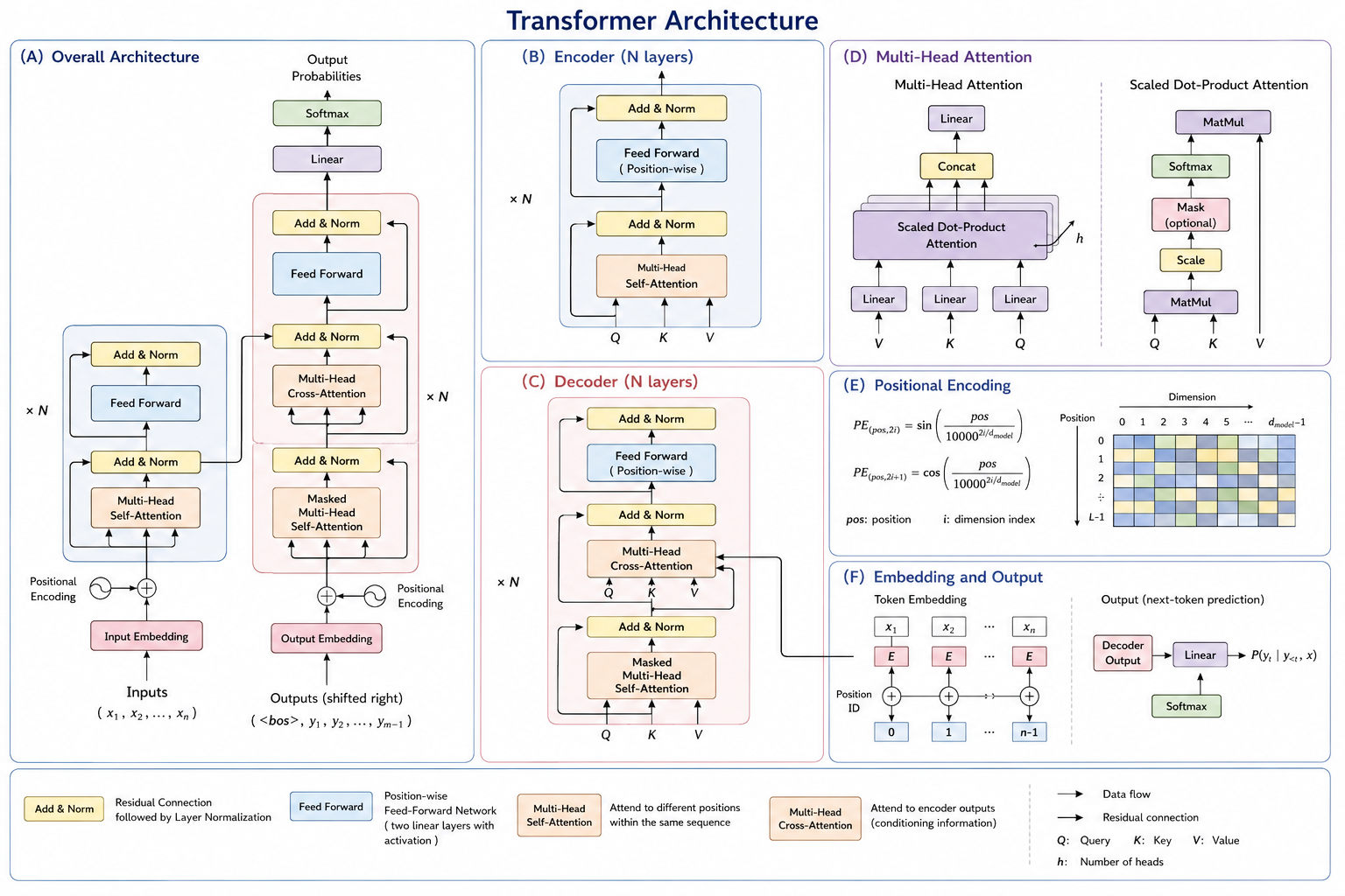
Figure 8.4: Transformer architecture. Input tokens are augmented with positional information, contextualized through stacked self-attention and feed-forward blocks, and aggregated for a downstream prediction or generation task.
Theoretical Foundations
Self-Attention Mechanism
The core innovation of Transformers is self-attention, which allows each time step to attend to all other time steps:
For each time step , compute:
- Query:
- Key: (for all time steps )
- Value: (for all time steps )
Attention weights:
where is the dimension of keys (scaled dot-product attention).
Output:
Intuition: Each position computes a weighted combination of all values, with weights based on query-key similarity. The network learns what to attend to.
The benefit of this all-to-all comparison is that a brief event can directly interact with a distant context, rather than passing through many recurrent updates. Its cost is the attention matrix: for $T$ tokens, standard attention compares $T^2$ pairs. This is manageable for short EEG windows but quickly becomes the dominant memory and compute cost for raw, long-duration recordings.
Multi-Head Attention
Using multiple attention heads in parallel:
where each head computes attention with different learned projections.
Benefits:
- Different heads learn different relationships
- Parallel computation
- More expressive than single attention head
Self-Attention Variants for Transformer Blocks
Attention variants modify which tokens may communicate and how the attention computation is stored. The standard global design is the most flexible, but it is not always the best default for EEG: it may be unnecessarily expensive for long recordings and can overfit when a small dataset permits every time step to attend to every other. The variants in Figure 8.4b address specific gaps—causal access for streaming prediction, local inductive bias for nearby EEG dynamics, sparse or linear computation for long sequences, and more efficient parameter sharing for deployment.
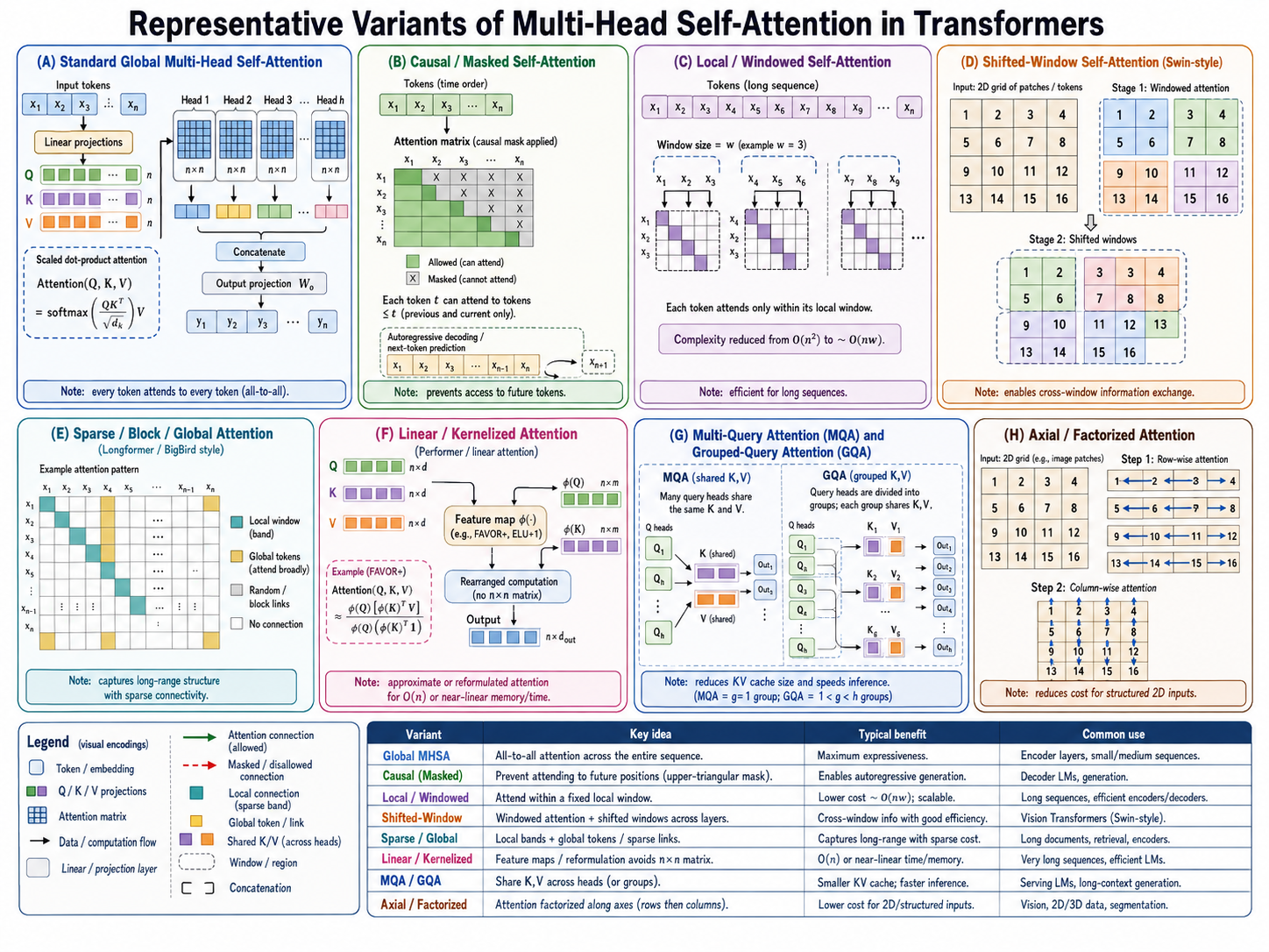
Figure 8.4b: Multi-head self-attention variants for Transformer blocks. Global attention connects every token; causal attention masks future tokens for online prediction; local and shifted-window attention reduce cost while retaining nearby and cross-window context; sparse/block-global attention reserves broad connections for selected tokens; linear/kernelized attention avoids explicitly forming the full attention matrix; multi-query/grouped-query attention shares key-value projections to reduce inference memory; and axial/factorized attention decomposes structured inputs along separate axes.
Choosing a variant for EEG. Use global attention as a short-window baseline when GPU memory permits. Use causal masking for real-time monitoring, where future samples must not leak into a prediction. Local, shifted-window, or sparse attention is often a better match for long recordings because nearby samples carry strong temporal continuity, while occasional global links can capture session-level context. Linear attention improves scalability but changes the attention approximation and should be checked for loss of fine temporal structure. Axial attention is most natural when tokens retain both a time and channel or frequency axis; it is less compelling for a simple one-dimensional sequence.
Positional Encoding
Since Transformers don't have inherent temporal ordering (all positions processed in parallel), positional information is added:
This ensures the model knows relative timing between samples.
Positional design is an EEG modeling decision, not a technical afterthought. Absolute encodings identify where a token appears in a fixed-length window, while relative encodings emphasize separation between events and can transfer more naturally across window lengths. When electrodes are represented as separate tokens, add spatial or channel embeddings as well; otherwise attention can learn temporal similarity without knowing which scalp locations produced it.
Transformer Block
A standard Transformer block contains:
- Multi-head self-attention
- Layer normalization
- Feed-forward network (two dense layers with ReLU)
- Layer normalization
- Residual connections (skip connections)
Stacking multiple blocks creates deep Transformers.
Residual paths let a block refine a representation without having to recreate it, and normalization keeps the scale of that refinement stable across depth. The feed-forward sublayer is equally important: attention mixes information between tokens, whereas the feed-forward network applies a nonlinear transformation to each contextualized token. Depth should be increased only when the dataset and validation strategy support it, since a deeper block stack can memorize subject- or session-specific patterns instead of generalizing affective structure.
Comparison with RNNs
| Aspect | Transformer | RNN/LSTM |
|---|---|---|
| Computation | Parallel for all time steps | Sequential |
| Memory access | Global (attends to all) | Local (previous hidden state) |
| Training speed | Fast (parallelizable) | Slow (sequential) |
| Maximum sequence length | Quadratic complexity | Linear complexity |
| Position information | Positional encoding | Built into recurrence |
| Long-range dependencies | Direct attention | Through hidden state chain |
Adaptation to EEG-based Affective Computing
Why Transformers for EEG?
Advantages:
- Efficient training: Parallel processing enables GPU acceleration
- Long-range dependencies: Direct attention to distant time steps
- Scaling: Effective with large datasets
- Transfer learning: Pre-trained models available
- Interpretability: Attention weights show what the model focuses on
Limitations:
- Quadratic complexity: Memory and time scale as where is sequence length
- Data requirements: Benefit from large datasets; can overfit on small data
- Limited local structure: Don't naturally exploit local temporal patterns
- Position encoding: Requires careful design for EEG temporal structure
EEG-Specific Considerations
The sequence-length problem motivates tokenization before model tuning. A token may represent a short raw-signal patch, a time-frequency patch, or a window-level feature vector; each choice defines what interactions attention can learn. Start by matching token duration to the fastest effect of interest, then choose an attention variant whose receptive field covers the slowest relevant temporal context.
Sequence Length Challenge:
- Standard EEG sessions: 30-300 seconds
- At 256 Hz: 7,680-76,800 samples
- Attention complexity: is prohibitive
Solutions:
- Chunking: Process 8-16 second windows (2,048-4,096 samples)
- Downsampling: Reduce sampling rate or aggregate samples
- Local attention: Attend only to nearby time steps
- Efficient attention variants: Sparse, linear, or kernel-based attention
Suitable Input Features
Representation Options
Input representation sets the Transformer’s inductive bias. Fine-grained tokens offer precise timing but make every attention layer expensive; coarser spectral or window-level tokens reduce length and add frequency structure, but may blur transient events. The most convincing comparison holds the total recording duration, subject split, and model capacity constant while varying only the tokenization scheme.
Option 1: Raw Time Series with Channel Embedding
# Shape: (sequence_length, n_channels)
# Example: (2048, 14)

# Process each channel independently:
input = EEG_signal  # (2048, 14)
# Transformer processes 2048 time steps
# Each time step includes 14-channel information
Advantage: No information loss Disadvantage: Long sequences may exceed memory limits
Option 2: Downsampled Signals
# Reduce temporal resolution
# Original: 256 Hz → Downsample to 64 Hz
# Shape: (512, 14)  # 2 seconds instead of 8

# Trade-off: Reduced computation but less temporal detail
Option 3: Spectral Features per Time Bin
# Pre-compute spectral features in short windows
# 1-second Hann windows with 50% overlap
# 8-second signal → 14 frequency-domain features per window
# Shape: (14, n_spectral_features)

# More efficient than raw signals
# Embeds frequency information
Option 4: Multi-Scale Representation
# Combine features at different time scales
# Fast scale (50 ms): Raw signal details
# Medium scale (500 ms): Local patterns
# Slow scale (2 sec): Global trends

# Concatenate multi-scale features
Preprocessing for Transformers
1. Careful Normalization
# Transformers are sensitive to scale
# Different normalization strategies:

# Global z-score (across entire session)
signal_norm = (signal - signal.mean()) / signal.std()

# Per-channel (handles channel-specific baselines)
for ch in range(n_channels):
    signal[:, ch] = (signal[:, ch] - signal[:, ch].mean()) / signal[:, ch].std()

# Per-segment (handles drift)
for seg in range(n_segments):
    signal[seg] = (signal[seg] - signal[seg].mean()) / signal[seg].std()
2. Handling Variable Sequence Lengths
# Transformers can handle variable lengths via masking:

# Pad shorter sequences:
from tensorflow.keras.preprocessing import sequence
padded_signal = sequence.pad_sequences(
    signals, maxlen=2048, padding='post', value=0
)

# Create attention mask (ignore padding):
mask = tf.cast(padded_signal != 0, tf.float32)
3. Segmentation Strategy
# For long sessions (300 seconds):
# Option A: Multiple chunks (8 sec each)
# Process each independently, aggregate predictions

# Option B: Hierarchical attention
# Lower level: Chunk-level attention
# Upper level: Cross-chunk attention

# Option C: Streaming processing
# Maintain context across chunks using cache
Network Architecture for EEG
The following architectures trade attention coverage against computation. Begin with a small encoder and a transparent tokenization baseline, then add depth, multi-scale processing, or sparse attention only when a failure mode is visible—for example, missed long-range context or memory limits. A larger architecture is not automatically more interpretable: attention maps should be evaluated alongside performance and physiological plausibility.
Minimal Transformer (Single Layer)
Input: (sequence_length, n_channels)
Example: (2048, 14)
   ↓
Positional Encoding
   ↓
Multi-Head Attention (8 heads)
   ↓
Feed-Forward Network
   ↓
Global Average Pooling
   ↓
Dense(64) → ReLU
   ↓
Output (emotion class)
Use when: Limited data or computational constraints.
Standard Transformer Encoder
Input: (sequence_length, n_channels)
Example: (2048, 14)
   ↓
Embedding / Positional Encoding
   ↓
[Transformer Block × 4]
   Each block:
   - Multi-Head Attention (8 heads)
   - Feed-Forward (512 hidden)
   - Layer Norm + Residual
   ↓
Global Average Pooling
   ↓
Dense(256) → ReLU → Dropout(0.3)
   ↓
Dense(64) → ReLU → Dropout(0.3)
   ↓
Output (emotion class)
Use when: Moderate-large data (2000+ samples) and resources.
Deep Transformer Stack
Input: (sequence_length, n_channels)
   ↓
Channel Embedding (project to d_model=256)
   ↓
Positional Encoding
   ↓
[Transformer Block × 12]  # 12 encoder layers
   - Multi-Head Attention (8 heads, d_model=256)
   - Feed-Forward (d_ff=1024)
   - Layer Norm + Residual
   ↓
Layer Norm
   ↓
Global Average Pooling
   ↓
Dense(512) → ReLU → Dropout(0.3)
   ↓
Dense(128) → ReLU → Dropout(0.2)
   ↓
Output (emotion class)
Use when: Large datasets (5000+ samples) and strong computational resources.
Efficient Transformer (Sparse Attention)
For very long sequences, use sparse attention patterns:
Input: (sequence_length, n_channels)
   ↓
Embedding / Positional Encoding
   ↓
[Sparse Transformer Block × 4]
   - Local attention (window=256)
   - Strided attention (stride=64)
   - Global attention (sampled)
   ↓
Global Average Pooling
   ↓
Output
Benefit: Reduces attention complexity from to or .
Multi-Scale Transformer
Processes different time scales:
Input: (sequence_length, n_channels)
   ↓
[Fine-grained branch]        [Coarse-grained branch]
↓                            ↓
Downsample 2x                Downsample 4x
Transformer (4 layers)       Transformer (4 layers)
↓                            ↓
Upsample                     Upsample
↓                            ↓
Concatenate + Fusion
   ↓
Output
Implementation Considerations
Practical Transformer performance is often dominated by choices outside the attention equation. Padding masks must prevent artificial padded values from attracting attention, positional information must align with the tokenization procedure, and subject-wise splits are essential because large models can memorize individual recording signatures. Record memory use, effective sequence length, and inference latency together with accuracy to make architecture comparisons meaningful.
Sequence Length and Memory
Memory usage for multi-head attention:
For batch=32, T=2048, d=256:
32 × 2048² × 256 / (10⁹) ≈ 33 GB (prohibitive!)
Solutions:
- Reduce sequence length: Process 512-1024 samples (2-4 seconds)
- Sparse attention: Only attend to nearby or sampled positions
- Gradient checkpointing: Trade memory for computation time
- Smaller hidden dimensions: d_model=128 instead of 256
- Smaller batch size: Trade parallelization for memory
Attention Head Configuration
| Num Heads | Hidden Dimension | Per-Head Dim | Typical Use |
|---|---|---|---|
| 1 | 64 | 64 | Minimal Transformer |
| 4 | 256 | 64 | Small models |
| 8 | 256 | 32 | Standard |
| 8 | 512 | 64 | Large models |
| 12 | 768 | 64 | BERT-like |
Constraint:
Positional Encoding Variants for EEG
Standard sinusoidal (default):
- Works well but doesn't learn temporal structure
Learnable positional embeddings:
pos_embedding = Embedding(max_seq_length, d_model)
Relative position encoding:
- Better for extrapolation beyond training length
Frequency-aware encoding:
# Incorporate EEG frequency bands into encoding
# Emphasize bands important for emotion (alpha, theta, etc.)
Example Application: Emotion Classification
Task
Classify 8-second EEG segments into emotional states.
Architecture
import tensorflow as tf
from tensorflow.keras import layers, Sequential

# Positional Encoding
class PositionalEncoding(layers.Layer):
    def __init__(self, d_model, max_len=2048):
        super().__init__()
        self.d_model = d_model

        # Compute positional encoding
        position = tf.range(max_len, dtype=tf.float32)[:, tf.newaxis]
        div_term = tf.exp(
            tf.range(0, d_model, 2, dtype=tf.float32) *
            -(tf.math.log(10000.0) / d_model)
        )

        pe = tf.zeros((max_len, d_model))
        pe_sin = tf.sin(position * div_term)
        pe_cos = tf.cos(position * div_term)
        # Interleave sin and cos

        self.register_buffer('pe', pe)

    def call(self, x):
        return x + self.pe[:x.shape[1]]

# Build model
model = Sequential([
    layers.Input(shape=(2048, 14)),

    # Project to hidden dimension
    layers.Dense(256),
    PositionalEncoding(d_model=256),

    # Transformer blocks
    layers.MultiHeadAttention(
        num_heads=8, key_dim=32, attention_axes=-2
    ),
    layers.LayerNormalization(),

    layers.Dense(512, activation='relu'),
    layers.Dense(256),
    layers.LayerNormalization(),

    # Classification
    layers.GlobalAveragePooling1D(),
    layers.Dense(128, activation='relu'),
    layers.Dropout(0.3),
    layers.Dense(num_emotions, activation='softmax')
])

model.compile(
    optimizer='adam',
    loss='categorical_crossentropy',
    metrics=['accuracy']
)
Preprocessing
import numpy as np

# 1. Load 8-second segments
segments = load_eeg_segments()  # (n_samples, 2048, 14)

# 2. Filter
from scipy import signal as scipy_signal
sos = scipy_signal.butter(4, [0.5, 40], btype='band', fs=256, output='sos')
segments_filtered = np.array([
    scipy_signal.sosfilt(sos, seg, axis=0)
    for seg in segments
])

# 3. Normalize (per-channel)
segments_norm = np.zeros_like(segments_filtered)
for ch in range(14):
    ch_data = segments_filtered[:, :, ch]
    segments_norm[:, :, ch] = (
        (ch_data - ch_data.mean()) / (ch_data.std() + 1e-6)
    )

# 4. Train
model.fit(segments_norm, emotion_labels,
          epochs=100, batch_size=32, validation_split=0.2)
Advantages and Disadvantages
| Aspect | Transformer | LSTM | CNN |
|---|---|---|---|
| Training parallelization | Excellent | Poor | Good |
| Sequence length | Global attention | Limited | Fixed window |
| Training speed | Fast | Slow | Medium |
| Memory efficiency | Poor (for long seqs) | Good | Good |
| Interpretability | Good (attention) | Low | Medium |
| Data requirements | High (10K+) | Medium (1K+) | Low-Medium (500+) |
| Real-time inference | Medium | Slow | Fast |
When to Use Transformers
Choose Transformers when:
- Large EEG datasets available (5000+ samples)
- Long sequences need to be processed
- You want attention visualization
- Transfer learning from pre-trained models desired
- Computational resources are available
Prefer alternatives when:
- Limited training data (<1000 samples)
- Computational resources constrained
- Sequence length very long (>10,000 samples)
- Real-time inference critical
- Simple local patterns sufficient
Best Practices
- Start with shorter sequences: 512-1024 samples, increase if needed
- Use efficient attention variants for long sequences
- Careful positional encoding: Critical for temporal structure
- Appropriate layer normalization: Helps with training stability
- Warm-up learning rate: Transformer training benefits from warm-up
- Gradient accumulation: Simulate larger batch sizes with limited memory
- Pre-training: Consider transfer learning from large EEG or EEG-like datasets
- Monitor attention patterns: Visualize what the model learns
Transfer Learning with Transformers
Pre-trained models available:
- EEG-specific: Models trained on large EEG datasets (e.g., EEGNet pre-trained)
- Audio-based: Might transfer (similar temporal patterns)
- Vision-based: Limited transfer (different modality)
Fine-tuning strategy:
# Load pre-trained model
model = load_pretrained_eeg_transformer()

# Freeze most layers
for layer in model.layers[:-2]:
    layer.trainable = False

# Fine-tune on your specific task
model.compile(optimizer='adam', loss='categorical_crossentropy')
model.fit(your_data, your_labels, epochs=10)
Summary
Transformers represent the frontier of deep learning for sequential data, including EEG. They offer:
- Computational efficiency through parallelization
- Strong performance on large datasets
- Interpretability via attention mechanisms
- Scalability to multiple layers
However, they require:
- Substantial training data (typically 5000+ samples)
- Careful sequence length management
- Sufficient computational resources
- Thoughtful positional encoding design
For EEG-based affective computing, Transformers are increasingly popular for:
- Large clinical or research datasets
- Applications requiring attention interpretability
- Transfer learning scenarios
- Session-level analysis
For smaller datasets or real-time applications, hybrid approaches or simpler models remain more practical.
Next: Hybrid Architectures and Advanced Models
References
- Vaswani, A., Shazeer, N., Parmar, N., et al. (2017). Attention is all you need. In NeurIPS.
- Devlin, J., Chang, M.-W., Lee, K., and Toutanova, K. (2019). BERT: Pre-training of deep bidirectional transformers for language understanding. In NAACL-HLT.
- Dosovitskiy, A., Beyer, L., Kolesnikov, A., et al. (2021). An image is worth 16×16 words: Transformers for image recognition at scale. In ICLR.
- Song, Y., Zheng, Q., Liu, B., and Gao, X. (2022). EEG conformer: Convolutional transformer for EEG decoding and visualization. IEEE Transactions on Neural Systems and Rehabilitation Engineering, 31, 710–719.
- Kostas, D., Aroca-Ouellette, S., and Rudzicz, F. (2021). BENDR: Using transformers and a contrastive self-supervised learning task to learn from massive amounts of EEG data. Frontiers in Human Neuroscience, 15, 653659.