Multi-Layer Perceptrons (MLPs) and Dense Networks
Overview
Multi-Layer Perceptrons represent the foundation of deep learning. They are fully connected neural networks where information flows in one direction—from input to output through hidden layers. While simple compared to modern architectures, MLPs remain effective for EEG-based affective computing when combined with appropriate feature engineering.
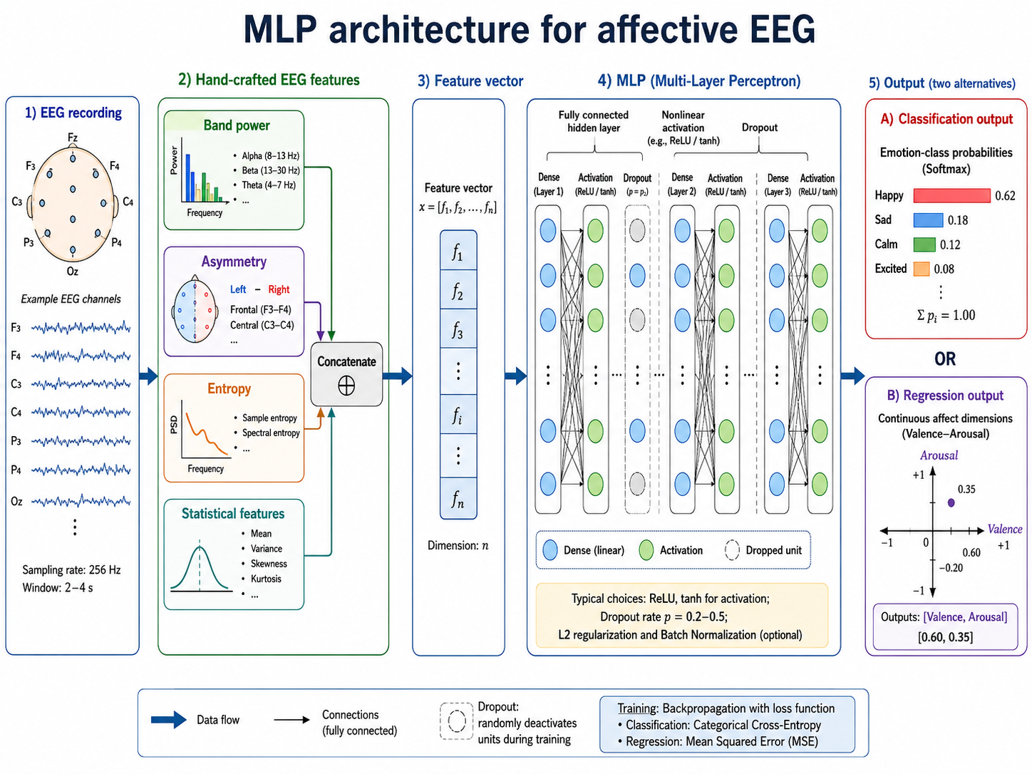
Figure 8.1: MLP architecture for affective EEG. A multilayer perceptron maps a fixed vector of engineered EEG features through dense nonlinear layers to a classification or regression output.
Theoretical Foundations
Architecture Structure
An MLP consists of:
- Input layer: Receives feature vectors of fixed dimension
- Hidden layers: Fully connected layers with non-linear activation functions
- Output layer: Produces predictions (emotion labels or regression values)
Each neuron computes:
where are inputs, are weights, is bias, and is an activation function (ReLU, tanh, sigmoid).
Activation Functions
- ReLU (Rectified Linear Unit): - Most common, computationally efficient
- Tanh: - Zero-centered, useful for hidden layers
- Sigmoid: - For binary classification outputs
Training
MLPs are trained using backpropagation with gradient descent, optimizing a loss function:
For classification: Cross-entropy loss For regression: Mean Squared Error (MSE)
Adaptation to EEG-based Affective Computing
Why MLPs for EEG?
Advantages:
- Simplicity: Easy to implement and understand
- Data efficiency: Require less data than convolutional or recurrent networks
- Speed: Fast inference, suitable for real-time applications
- Proven effectiveness: Solid baseline performance with good features
Limitations:
- Require manual feature engineering
- Cannot leverage raw signal structure
- Lose spatial/temporal relationships
- May not capture complex patterns without very deep networks
Typical Pipeline
Raw EEG → Preprocessing → Feature Extraction → MLP → Emotion Label
           (Filtering,        (Frequency,      (Dense (Valence/
           Normalization)     Spectral,        Layers) Arousal)
                              Statistical)
Suitable Input Features
Feature Categories for EEG
1. Frequency Domain Features
Power Spectral Density (PSD) in standard bands:
- Delta (0.5–4 Hz): Deep sleep, meditation
- Theta (4–8 Hz): Relaxation, memory
- Alpha (8–13 Hz): Relaxed alertness
- Beta (13–30 Hz): Active thinking, problem-solving
- Gamma (30–100 Hz): Attention, cognitive processing
Band Power Ratios:
- Alpha/Theta ratio: Relaxation indicator
- Beta/Alpha ratio: Engagement level
- (Alpha_right - Alpha_left) / (Alpha_right + Alpha_left): Frontal asymmetry
2. Statistical Features
- Spectral moments: Mean frequency, median frequency, spectral entropy
- Time-domain statistics:
- Mean, variance, skewness, kurtosis
- Peak-to-peak amplitude
- Approximate entropy
3. Differential Asymmetry (DA)
Asymmetric frontal activity correlates with emotional valence.
4. Relative Power
Normalizes power across individuals and sessions.
Feature Dimensionality
For a typical 14-channel EEG system:
- 5 frequency bands × 14 channels = 70 PSD features
- Plus ratios, asymmetries, and statistical features
- Often results in 100–200 dimensional feature vectors
Preprocessing Pipeline
Step 1: Raw Signal Acquisition
EEG Recording → 14-64 channels at 250-1000 Hz
Step 2: Artifact Removal
Objectives: Remove non-brain electrical activity
Methods:
Filtering:
- High-pass filter (0.5-1 Hz) removes DC drift
- Low-pass filter (40-100 Hz) removes high-frequency noise
- Notch filter (50/60 Hz) removes electrical line noise
Independent Component Analysis (ICA):
- Identifies and removes EOG (eye movement), EMG (muscle) components
Automatic artifact detection:
- Amplitude thresholding: Remove samples exceeding ±100-200 μV
- Variance-based methods
Step 3: Segmentation
Objectives: Create fixed-length windows for analysis
- Window size: 4–10 seconds (typically 1000–2500 samples at 250 Hz)
- Overlap: 50% or none, depending on desired temporal granularity
- Emotional state assumption: Emotion is relatively stable within window
Step 4: Feature Extraction
for each segment:
    1. Apply bandpass filters for each frequency band
    2. Compute PSD (using Welch's method or FFT)
    3. Calculate statistical features
    4. Compute asymmetry and ratio features
    5. Concatenate all features
Step 5: Normalization
Global normalization (across entire dataset):
Where and are computed on training data.
Per-session normalization (handles inter-session variability):
x_norm = (x - x.mean()) / x.std() # For each session
Network Architecture for EEG
Simple Architecture (Baseline)
Input (128 features)
  ↓
Dense(256, ReLU)
  ↓
Dropout(0.5)
  ↓
Dense(128, ReLU)
  ↓
Dropout(0.3)
  ↓
Output (emotion label)
Rationale: Moderate depth prevents overfitting on limited EEG datasets while capturing feature interactions.
Deeper Architecture (High-capacity)
Input (128 features)
  ↓
Dense(512, ReLU) → Batch Norm → Dropout(0.5)
  ↓
Dense(256, ReLU) → Batch Norm → Dropout(0.4)
  ↓
Dense(128, ReLU) → Batch Norm → Dropout(0.3)
  ↓
Dense(64, ReLU) → Batch Norm → Dropout(0.2)
  ↓
Output (emotion label)
When to use: Larger datasets (1000+ samples) or multi-task learning.
Sparse Architecture (Limited Data)
Input (128 features)
  ↓
Dense(128, ReLU)
  ↓
Dropout(0.3)
  ↓
Output (emotion label)
When to use: Limited training data (<500 samples).
Implementation Considerations
Handling Imbalanced Data
Emotional states are often imbalanced. Strategies:
- Class weighting: Assign higher loss weight to minority classes
- Oversampling: Replicate minority class samples
- Undersampling: Remove majority class samples
- SMOTE: Synthetic Minority Oversampling Technique
Regularization Techniques
Dropout: Randomly deactivate neurons during training (prevents co-adaptation)
model.add(Dropout(0.5)) # Deactivate 50% of neurons
L2 Regularization (Weight decay):
Controls model complexity by penalizing large weights.
Early stopping: Monitor validation loss, stop when it plateaus
Hyperparameter Tuning
| Hyperparameter | Typical Range | EEG Best Practice |
|---|---|---|
| Hidden units | 64–1024 | 128–512 |
| Number of layers | 2–5 | 2–4 |
| Dropout rate | 0.2–0.7 | 0.3–0.5 |
| Learning rate | 0.0001–0.1 | 0.001–0.01 |
| Batch size | 16–128 | 32–64 |
| Optimizer | Adam, SGD | Adam |
Cross-Subject Generalization
Challenge: Models trained on one subject's data may not generalize to others.
Solutions:
- Subject-independent training: Pool data from multiple subjects
- Transfer learning: Pre-train on one domain, fine-tune on target
- Domain adaptation: Reduce subject-specific bias
- Leave-one-subject-out (LOSO) validation: Realistic performance estimate
Example Application: Emotion Classification
Task
Classify EEG signals into emotional states: Positive, Neutral, Negative
Architecture
from tensorflow.keras import Sequential, layers

model = Sequential([
    layers.Input(shape=(128,)),  # 128 hand-crafted features

    layers.Dense(256, activation='relu'),
    layers.BatchNormalization(),
    layers.Dropout(0.5),

    layers.Dense(128, activation='relu'),
    layers.BatchNormalization(),
    layers.Dropout(0.3),

    layers.Dense(3, activation='softmax')  # 3 emotion classes
])

model.compile(
    optimizer='adam',
    loss='categorical_crossentropy',
    metrics=['accuracy']
)
Preprocessing Pipeline
# 1. Load raw EEG
signal = load_eeg_data()  # (n_channels=14, n_samples=250000)

# 2. Filter
signal = bandpass_filter(signal, 0.5, 40)

# 3. Segment
segments = segment_signal(signal, window=2048, overlap=0.5)

# 4. Extract features
features = []
for segment in segments:
    psd = compute_psd(segment, freq_bands=[0.5, 4, 8, 13, 30, 40])
    stats = compute_statistics(segment)
    asymmetry = compute_asymmetry(psd, channels)
    feat_vec = np.concatenate([psd, stats, asymmetry])
    features.append(feat_vec)

# 5. Normalize
features = (features - features.mean(axis=0)) / features.std(axis=0)

# 6. Train
model.fit(features, labels, epochs=100, batch_size=32)
Advantages and Disadvantages
| Aspect | MLPs | CNNs | RNNs |
|---|---|---|---|
| Feature engineering | Requires manual features | Automatic extraction | Automatic extraction |
| Temporal information | Lost (if averaged) | Implicit in features | Explicit (sequential) |
| Spatial relationships | Not exploited | Exploited locally | Not leveraged |
| Computational cost | Low | Medium | High |
| Data requirements | Low-medium | Medium-high | High |
| Interpretability | High (feature importance) | Medium | Low |
Summary
Multi-Layer Perceptrons provide a solid foundation for EEG-based affective computing when:
- Features are well-engineered
- Computational resources are limited
- Data is relatively small
- Real-time performance is critical
The key to success with MLPs lies in feature engineering—extracting frequency-domain features, statistical properties, and asymmetries that capture emotional correlates in EEG signals.
For many modern applications, however, automatic feature learning through CNNs or RNNs often yields better performance. MLPs work best as part of a pipeline after initial feature extraction or as a baseline for comparison.
Next: Convolutional Neural Networks for EEG
References
- Rumelhart, D. E., Hinton, G. E., and Williams, R. J. (1986). Learning representations by back-propagating errors. Nature, 323, 533–536.
- Cybenko, G. (1989). Approximation by superpositions of a sigmoidal function. Mathematics of Control, Signals and Systems, 2, 303–314.
- Hornik, K., Stinchcombe, M., and White, H. (1989). Multilayer feedforward networks are universal approximators. Neural Networks, 2(5), 359–366.
- Glorot, X., Bordes, A., and Bengio, Y. (2011). Deep sparse rectifier neural networks. In AISTATS.
- Srivastava, N., Hinton, G., Krizhevsky, A., Sutskever, I., and Salakhutdinov, R. (2014). Dropout: A simple way to prevent neural networks from overfitting. JMLR, 15, 1929–1958.
- Zheng, W.-L., and Lu, B.-L. (2015). Investigating critical frequency bands and channels for EEG-based emotion recognition with deep neural networks. IEEE Transactions on Autonomous Mental Development, 7(3), 162–175.