Neural Ordinary Differential Equations for Affective EEG

Neural ordinary differential equations (Neural ODEs) represent hidden-state evolution in continuous time. Instead of specifying a fixed stack of discrete layers or a fixed recurrent update for every sample, they learn a differential equation whose solution evolves between observation times. This is useful for EEG when sampling is irregular, observations are missing, affect is modeled as a continuous latent process, or a system must reason about dynamics at a chosen temporal resolution.

Neural ODEs are not a claim that EEG follows one simple deterministic physical equation. They are a modeling tool: a learned continuous-time approximation with assumptions about smoothness, observability, and numerical integration that must be tested against simpler sequence baselines.

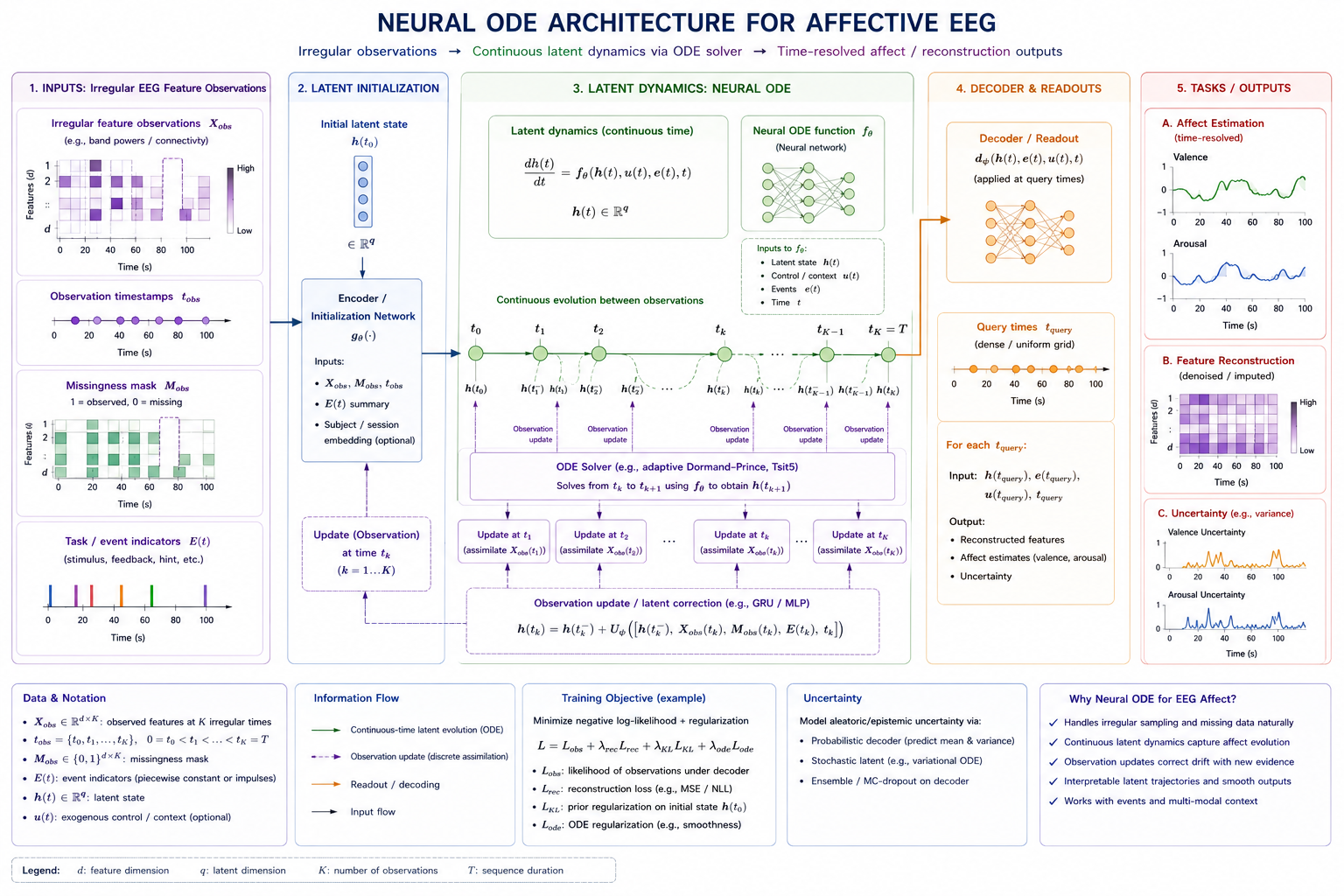
Figure 8.13: Neural ODE architecture for affective EEG. A continuous-time latent state is updated from EEG observations and evolved by a learned differential equation before being decoded into affective trajectories or signal predictions.

Continuous-Time Latent Dynamics

A Neural ODE specifies the derivative of a latent state $z(t)$ :

$\frac{d z(t)}{dt} = f_\theta(z(t), t, u(t)),$

where $f_\theta$ is a neural network and $u(t)$ can include EEG features, stimulus context, task events, or other controls. Given an initial state $z(t_0)$ , an ODE solver produces

$z(t_1) = z(t_0) + \int_{t_0}^{t_1} f_\theta(z(t), t, u(t))\,dt.$

A decoder maps $z(t)$ to a continuous affect estimate, class distribution, reconstructed EEG feature, or control value. The integration step is selected by a solver and does not need to match the raw EEG sampling interval; this can be an advantage for irregular observations, but it also introduces solver accuracy and latency tradeoffs.

Core Architectures and Variations

Variant	Main idea	EEG-relevant use	Main caution
Neural ODE	Deterministic latent dynamics	Smooth continuous state tracking	May underrepresent abrupt events or stochasticity
Latent ODE	Infer initial latent state from irregular observations, then evolve continuously	Sparse or irregular annotations and missing windows	Posterior inference can be difficult
ODE-RNN	Recurrent updates at observations plus ODE evolution between them	Longitudinal or event-driven recordings	More moving parts and tuning choices
Neural CDE	Drives latent dynamics with a continuous interpolation of observed path	Irregular multichannel time series with informative observation paths	Interpolation and control path must be justified
Augmented Neural ODE	Adds latent dimensions to avoid restrictive flow topology	More expressive continuous transformations	Higher cost and weaker interpretability
Neural SDE	Adds stochastic diffusion to latent dynamics	Uncertainty and random fluctuations	Harder training and calibration
Continuous normalizing flow	Uses an ODE to transform probability densities	Likelihood modeling and continuous generative representations	Computationally demanding

Latent ODE and ODE-RNN

Latent ODE models encode irregular observations into an initial distribution over $z(t_0)$ , then solve a continuous-time dynamics model. ODE-RNNs instead alternate discrete recurrent updates when measurements arrive with continuous ODE evolution in gaps. These approaches are relevant when wearable EEG contains dropped packets, variable segment lengths, or sparse affect labels.

Example scenario: A user wears a mobile EEG device during an extended task. Signal-quality checks produce irregular valid windows, and occasional self-reports arrive at nonuniform times. An ODE-RNN updates its latent state at valid windows, evolves between them, and predicts a continuous workload trajectory with uncertainty. Evaluation uses chronological held-out periods and compares against a masked Transformer and a standard RNN using the same valid observations.

Neural Controlled Differential Equations

Neural CDEs treat a multivariate observation path $X(t)$ as a control signal:

$dz(t) = f_\theta(z(t))\, dX(t).$

The path can include EEG features, timestamps, missingness indicators, peripheral physiology, task events, and context. CDEs are particularly natural when the pattern of observations and timing carries information. For EEG, use a declared interpolation scheme and ensure that a causal deployment does not use future samples to construct the control path.

Neural SDEs and Stochastic Dynamics

A Neural SDE adds a stochastic term:

$dz(t) = f_\theta(z(t), t)dt + g_\theta(z(t), t)dW_t,$

where $W_t$ is a Wiener process. This can represent uncertainty, unobserved perturbations, and variable affective fluctuations more flexibly than a deterministic ODE. It is useful only when uncertainty is evaluated and calibrated; adding noise without a probabilistic objective does not make a model more realistic.

Incorporating Graph Structure

EEG latent dynamics can respect spatial or functional graph structure. Let $H(t)$ contain node states for electrodes or source regions and let $A$ be an adjacency matrix. A graph Neural ODE can define

$\frac{dH(t)}{dt} = f_\theta(H(t), A, t),$

where $f_\theta$ is a graph convolution, graph attention, or directed message-passing network. This supports continuously evolving connectivity-aware representations rather than independently applying a GNN at fixed windows.

Useful directions include:

Graph Neural ODEs over electrode or source nodes for continuous spatio-temporal EEG representations;
Dynamic graph ODEs in which $A(t)$ changes with task phase or inferred connectivity;
Directed or causal graph ODEs that constrain messages according to a validated directed graph, with careful causal interpretation;
Geometry-aware graph dynamics that use electrode coordinates or source meshes;
and multimodal controlled graph ODEs driven by EEG, peripheral signals, task events, and user actions.

Graph structure improves inductive bias only when it is justified. A learned dynamic adjacency can overfit small datasets, while a fixed connectivity graph can be wrong for a given subject or condition. Compare graph and non-graph continuous-time baselines under the same split.

Affective EEG Applications

Neural ODEs are especially relevant to:

continuous valence-arousal, workload, or stress tracking;
affect dynamics with irregular self-reports or missing EEG intervals;
personalization through subject-specific initial states or lightweight dynamic adapters;
online BCI state estimation where prediction update rate differs from sensor sampling rate;
longitudinal modeling across sessions, with time-aware drift components;
and latent neural-field dynamics coupled to operator-learning or source-imaging models.

For short, fixed, trial-level classification, a conventional CNN, Transformer, or recurrent model is often simpler and easier to validate. Continuous-time models are most justified when observation timing, gaps, dynamics, or solver-controlled resolution are part of the task itself.

Training, Solvers, and Stability

Training differentiates through an ODE solver using direct backpropagation, adjoint methods, or checkpointed variants. Solver tolerance, method, maximum step size, and function-evaluation budget affect accuracy, memory, compute, and gradients. They are model hyperparameters and should be selected on validation data.

Stiff dynamics, exploding trajectories, and high solver cost can arise with noisy EEG. Practical stabilizers include bounded vector fields, spectral normalization, regularization of Jacobians or kinetic energy, fixed-step solvers for predictable latency, and hybrid models that reset or update the state at observed event boundaries.

For online deployment, report warm-up, state initialization, update rate, solver latency, and behavior after missing data. A noncausal smoother or an interpolation using future observations invalidates a strict real-time claim.

Evaluation

Evaluate both predictive quality and dynamic behavior:

Claim	Evaluation
Continuous affect tracking	Time-resolved error, concordance, calibration, and lag-aware correlation
Irregular-data handling	Performance under controlled missingness and real dropped-window patterns
Temporal transfer	Chronological and cross-session held-out evaluation
Dynamic plausibility	Stability, trajectory smoothness, event response, and sensitivity to initial state
Graph contribution	Graph ODE versus matched non-graph ODE and discrete-time GNN baselines
Efficiency	Solver function evaluations, memory, latency, and energy use

A smooth trajectory is not necessarily correct. Compare against persistence, state-space, RNN, SSM, and Transformer baselines, and inspect whether the model responds appropriately to genuine events instead of smoothing them away.

Practical Recommendations

Use Neural ODEs when continuous time, irregular sampling, or latent dynamics are core to the problem; otherwise begin with discrete-time baselines.
Include timestamps, missingness masks, signal-quality indicators, and task events explicitly rather than expecting the ODE to infer them.
Choose causal interpolation and fixed solver budgets for real-time systems.
Test deterministic ODE, CDE, and SDE variants only when their additional assumptions match the data and desired uncertainty behavior.
Add graph structure when electrode or source relations are independently justified and evaluate it against a non-graph continuous-time model.
Report solver, tolerance, step-size, state dimension, initialization, and numerical-stability settings for reproducibility.

References

Chen, R. T. Q., Rubanova, Y., Bettencourt, J., and Duvenaud, D. (2018). Neural ordinary differential equations. Advances in Neural Information Processing Systems, 31.
Rubanova, Y., Chen, R. T. Q., and Duvenaud, D. (2019). Latent ODEs for irregularly-sampled time series. Advances in Neural Information Processing Systems, 32.
Kidger, P., Morrill, J., Foster, J., and Lyons, T. (2020). Neural controlled differential equations for irregular time series. Advances in Neural Information Processing Systems, 33.
Dupont, E., Doucet, A., and Teh, Y. W. (2019). Augmented neural ODEs. Advances in Neural Information Processing Systems, 32.
Liu, X., et al. (2020). Neural SDE: Stabilizing neural ODE networks with stochastic noise. arXiv:1906.02355.
Poli, M., Massaroli, S., Park, J., et al. (2019). Graph neural ordinary differential equations. arXiv:1911.07532.

8.12 Neural Ordinary Differential Equations